A consistent dataset for the net income distribution for 190 countries and aggregated to 32 geographical regions from 1958 to 2015

Data on income distributions within and across countries are becoming increasingly important for informing analysis of income inequality and understanding the distributional consequences of climate change. While datasets on income distribution collected from household surveys are available for multiple countries, these datasets often do not represent the same concept of inequality (or income concept) and therefore make comparisons across countries, over time and across datasets difficult. Here, we present a consistent dataset of income distributions across 190 countries from 1958 to 2015 measured in terms of net income. We complement the observed values in this dataset with values imputed from a summary measure of the income distribution, specifically the Gini coefficient. For the imputation, we use a recently developed nonparametric principal-component-based approach that shows an excellent fit to data on income distributions compared to other approaches. We also present another version of this dataset aggregated from the country level to 32 geographical regions. Our dataset is developed for the purpose of calibrating models such as integrated human–Earth system models with detailed data on income distributions. This dataset will enable more robust analysis of income distribution at multiple scales. The latest version of our data are available on Zenodo: https://doi.org/10.5281/zenodo.7093997 (Narayan et al., 2022b).

1 Introduction

Data on income distributions are important for understanding trends in global and regional income inequality. These data are also routinely used to train models that project income distributions into the future (Fujimori et al., 2020; Hallegatte and Rozenberg, 2017; Hughes, 2019; Hughes et al., 2009; Soergel et al., 2021; Van Der Mensbrugghe, 2015). In the climate literature, long-term projections of within-country income distribution have been used to inform analyses of how the impacts of climate change may affect inequality and poverty (Hallegatte and Rozenberg, 2017; Jafino et al., 2020). Income distribution data are generally collected through national and local household surveys. The most prominent sources of national-level income distribution data are the datasets presented by the World Bank through the PovCal tool (Bank, 2015) and the income distribution datasets available from the Luxembourg Income Study (LIS) (Ravallion, 2015; Smeeding and Grodner, 2000). Both these datasets present useful time series of income distribution for income groups such as deciles, based on multiple household surveys.

While these datasets have been widely used, they are subject to certain limitations. The definition of income in these datasets is often not the same, making comparisons across countries and datasets difficult (Smeeding and Latner, 2015). For example, the PovCal dataset has mixed observations for net income and consumption for the same country in different years. Such inconsistencies can occur because the underlying surveys in different years might have been conducted to measure different concepts of inequality (hereafter referred to as income concepts). The two income concepts that these data tend to use are the following.

• i.

  Post-tax income, disposable income or net income. This measure is defined as employee income plus income from firms (self-employment) plus income from rentals (excluding any payments), property income (these are generally capital gains and include dividends) and current transfers received (these include insurance benefits and employer contributions) less transfers paid (taxes paid and employee contributions). This is the concept of income recommended by the Canberra group for the international comparison of incomes (UNECE, 2011).

• ii

  Consumption. This measure is the sum of food consumption plus non-food consumption plus durable goods purchases (expenditure value minus the cost of repairs) plus housing expenditures (rent, mortgage payments) less any payments made (taxes, loan payments, asset purchases, etc.). This is the concept of income recommended by Deaton and Zaidi (2002) for welfare measurement.

Temporal and spatial coverage of the data is another issue. The LIS dataset provides consistent data on the net income distribution. However, these data are only available for 50 countries from 1980 to 2016. The PovCal dataset provides data for a considerably higher number of countries (165) compared to the LIS. However, the data are a combination of net income and consumption-based observations (net income distribution data for 73 countries and consumption distribution data for 118 countries).

Previous studies that have made use of these datasets for analysis or for modeling income distributions have treated these income concepts as interchangeable (Rao et al., 2019; Pachauri, 2020). Moreover, for countries where no survey data on income distributions are available, studies have used simple methods, e.g., using a summary measure of income distribution such as the Gini coefficient in combination with a parametric functional form such as a lognormal distribution to impute the within-country or within-region income distribution (Fujimori et al., 2020; Rao et al., 2019; Shorrocks and Wan, 2008; Soergel et al., 2021).

There have been efforts to generate consistent datasets of the income distribution. However, these efforts have been limited to local or regional data. For example, Frank (2009) generated a consistent dataset of income distribution metrics for a single income concept for the 50 US states. That particular study builds on previous studies that compiled data for the US states (Piketty and Saez, 2003). At the national level, there have been some efforts to produce standardized datasets of income inequality, but they have generally been limited to summary metrics of the income distribution such as the Gini coefficient (Babones and Alvarez-Rivadulla, 2007). Lanker and Milanovic (Lakner and Milanovic, 2016) developed a useful time series of income deciles across countries, which is a combination of data from the LIS, PovCal and other sources. However, this dataset is still a combination of different income concepts and has a limited temporal time series (the dataset only extends to the year 2013).

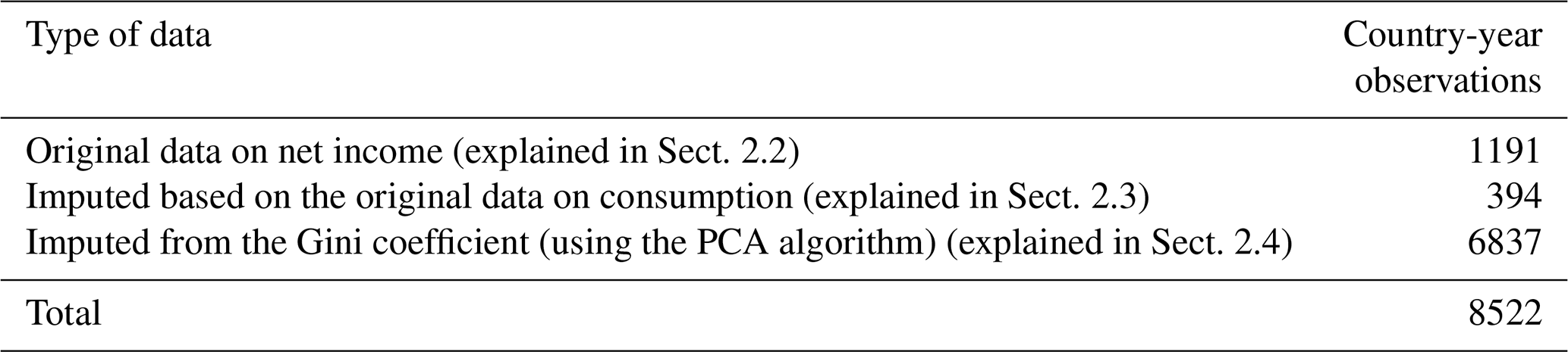
In this study we present a consistent dataset on national income distributions that represents a single income concept, i.e., net income. This dataset contains a total of 8522 data points of income deciles across 190 countries. It is constructed by first choosing net income decile data observations from all available sources for all available countries (1191 observations). For countries that only have consumption distribution data, we impute the net income distribution using a regression-based approach (494 observations). For countries and years where no data on income distribution are available, we impute income deciles using the Gini coefficient combined with a principal component analysis (PCA)-based method that provides a better fit to data than existing methods (6837 observations). This PCA-based method was recently developed as a nonparametric approach to projecting income distribution (Narayan et al., 2023). While this method was primarily used for generating estimates of future income distributions, the same was also validated against historical data (as described in the sections below) and hence was selected as a valid method to perform imputations. We note that the PCA-based imputation provides the maximum number of observations in the dataset.

One intended use of this dataset is to initialize income distribution variables in the Global Change Analysis Model (GCAM) (Calvin et al., 2019). GCAM is a global integrated model of the energy, land, water, climate and socioeconomic systems that produces projections for several economic, climatological and physical system variables for 32 geopolitical regions. Hence, we also present income distributions for these 32 aggregated regions, in addition to the 190 countries. We use an aggregation method that takes into account cross-country inequality within a region in addition to within-country inequality.

This dataset can be used to train projection models for income distribution across different scales and, given the consistent income concept represented, can also be used to understand trends within and across countries and regions. While these data are generated to enable modeling of the income distributions in GCAM, they can be used to train any model for projecting income distributions.

2 Dataset construction

We explain our approach for the dataset construction in detail in the sections below. To summarize, we used the following steps.

• a.

  We first identified observations by the country and year of net income deciles from all available datasets (LIS, PovCal and individual research studies). In doing so, we prioritized the LIS dataset over all other datasets given its high data quality on the net income distribution. Our selection process is explained in Sect. 2.1 and 2.2 below.

• b.

  For countries and years in which there were no net income data but consumption data were available, the net income distribution was imputed from the consumption distribution using a regression-based approach. This is explained in Sect. 2.3.

• c.

  Where there were no net income or consumption data but the Gini coefficient, a summary metric of the income distribution, was available, we imputed the net income distribution from the summary measure using a PCA-based approach. This is explained in Sect. 2.4.

Note that point (c) above yields the maximum number of data points in our final dataset. Table 1 below summarizes the coverage of our dataset.

Table 1 Summary of the data points covered in our dataset.

2.1 Literature review and data selection from available household survey data

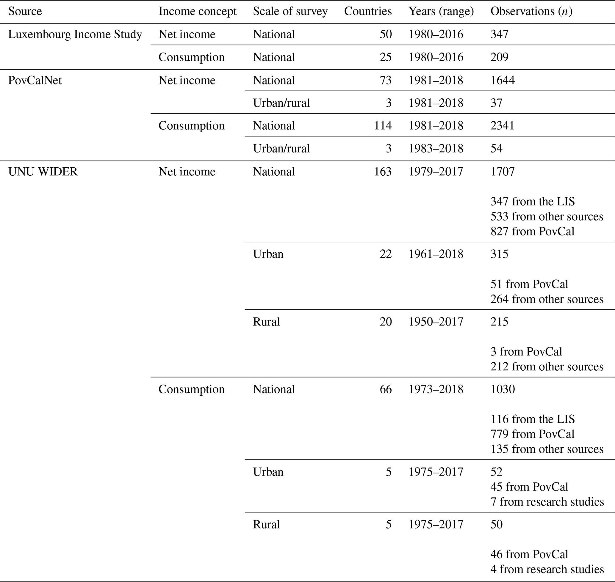
We first conducted a literature review to identify sources of national-level data on income distributions for as many countries as possible. There are three main datasets available from the LIS (Ravallion, 2015; Smeeding and Grodner, 2000), the World Bank (whose data on income distributions are available through the PovCalNet tool) (Bank, 2015) and UNU WIDER (United Nations University World Institute for Development Economics Research) (which compiles data from different sources, including the LIS, PovCal and other research studies) (Wider, 2008). Each dataset contains income distribution data for different income concepts such as net income and consumption, based on nationally representative surveys that may also represent subgroups of the population (e.g., urban vs. rural). These data are sometimes supplemented with data from research studies, and they use different equivalence scales to convert from household to per capita income. We first evaluated data availability for net income deciles based on these criteria (income concept, scale, temporal coverage and spatial coverage).

In Table 2, we summarize these datasets differentiated by these criteria. Since the UNU WIDER dataset is a compilation of data sources (i.e., the LIS, PovCal and others), we also identified the number of observations (country years) in the UNU WIDER data derived from each source. Table S1 in the Supplement summarizes some of the other studies which were used in the collection of data for the UNU WIDER database.

We are primarily interested in decile-level income distributions derived from household surveys. Given our criteria for data selection, we limited our data collection to the datasets mentioned above. For example, we did not use the Standardized World Income Inequality Database (Solt, 2020) since it only includes the Gini coefficient and not a full distribution by income groups (such as deciles). Similarly, we did not use the World Inequality Database (Chancel and Piketty, 2021), since this dataset is not based on household survey data (this database uses a distributed national account methodology). However, as more detailed datasets become available, they can be included in our dataset.

Table 2 Summary of coverage by data source.

We also evaluated access to microdata (i.e., underlying household-level data from household surveys) for each of these datasets, since detailed microdata allow us to validate and understand how the different income distributions for different income concepts were arrived at. Of all the datasets evaluated, we found that the LIS database has the most access to microdata via the METIS tool (https://www.lisdatacenter.org/frontend, last access: 31 August 2023).

The PovCal database maintained by the World Bank has the highest coverage geographically and temporally in terms of observations. PovCal uses the disposable-income data from the LIS for high- and middle-income countries and uses household survey data for consumption and disposable income for low-income countries. The scales of the surveys are mostly national other than India, China and Indonesia, where distribution data from separate rural and urban surveys are available. Mean and median values of the income concepts are available in USD 2011 PPP (purchasing power parity), converted using country-specific conversion factors.

PovCal sometimes combines data of different types, even within countries. For example, for China, PovCal uses income data in the early years up to 1990 and then switches to consumption data. Moreover, the microdata for PovCal are not readily available.

UNU WIDER releases quality scores of individual datasets. It classifies the LIS database as “High quality”, due especially to the availability of metadata, and classifies the PovCal dataset as “Average quality”. Figure 1 below shows the income distributions by deciles for different countries for different income concepts from the UNU WIDER dataset.

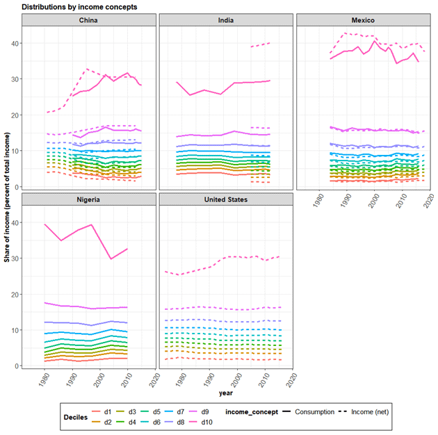
Figure 1 Income distributions across countries (facets) for different deciles (color) for different income concepts (line types) from the UNU WIDER dataset.

2.2 Selection of the income concept and scheme for selection of data points

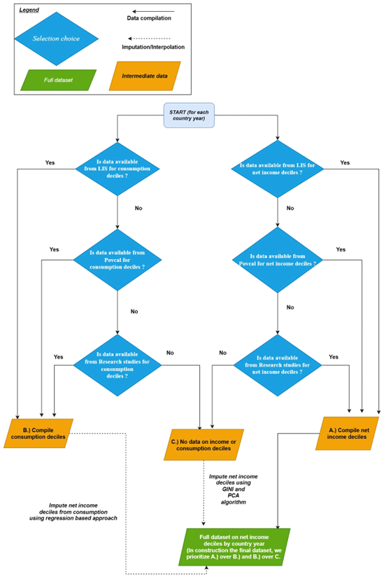
We construct a dataset that represents solely net income based on the same per capita equivalence scale. The per capita equivalence scale is calculated using total household income divided by the household size assuming equal sharing of income. Our process, summarized in Fig. 2, improves upon other attempts to construct income distribution datasets from different sources (Rao and Min, 2018; Rao et al., 2019), since the previous studies used the income concept from different datasets interchangeably. We primarily select observations for net income deciles across countries from the LIS, given the high quality of data available from that dataset. We begin by compiling separate datasets of the income distribution for net income and consumption. In the construction of both these datasets, we prioritize data points from the LIS. If no data were available from the LIS for a country-year observation, we selected an observation of net income or consumption from the PovCal database. Finally, if data were not available from that database, we rely on income distribution data from other research studies available from the UNU WIDER database. Note that, when selecting values across multiple research studies, we select values based on the rating assigned by the UNU WIDER database to the studies. All data are selected for the equivalence scale applied in the WIDER dataset, in which household income was converted to per capita units by dividing the household income by the household size assuming equal sharing of income. Note that, when selecting data points, the WIDER dataset presents data in multiple equivalence scales. This enabled us to select data that represent a single equivalence scale.

Thus, at this stage, we compiled two different datasets, one that represents net income distribution for countries across time and another that represents consumption for the same countries. Now, we prioritize the selection of net income distribution values over consumption for each country year.

Where data are only available for the consumption distribution, we convert the consumption data to net income data (as explained in Sect. 2.3 below) using a regression approach to generate a harmonized dataset of net income deciles. Where necessary, we aggregated data sources across different survey scales (urban vs. rural) using a population-weighted average.

Figure 2 summarizes our data selection approach.

Figure 2 Summary of the data selection approach for each country-year observation.

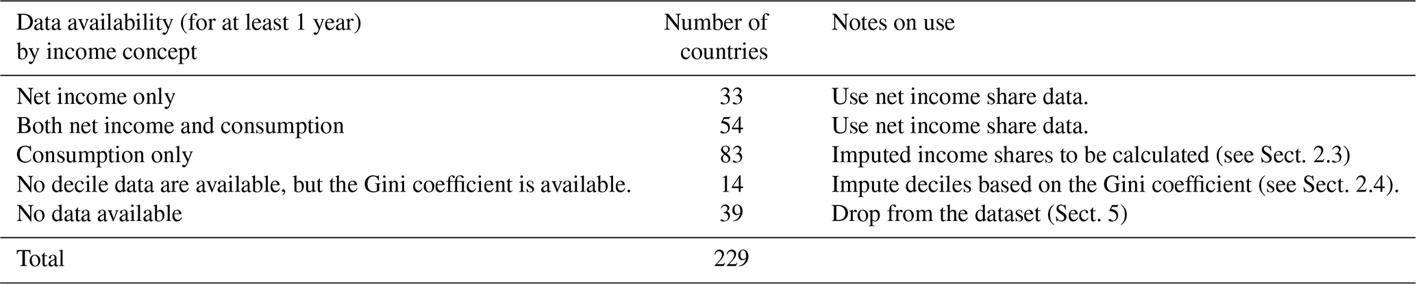
Based on the above, we evaluated data coverage for the 229 countries we are targeting. The geographical boundaries of the 32 GCAM regions are defined based on these 229 countries (countries with their corresponding regions are listed in Table S2 in the Supplement). We identified observations after the selection above for four categories, i.e., countries where we have net income data for at least 1 year, countries where we had both net income and consumption distribution data for at least 1 year (in the case of these countries, we selected the net income distribution value for deciles), countries where we had only consumption data and countries where there were no data (these countries only had data on aggregate measures of inequality, such as the Gini coefficient, but no data on income deciles). Table 3 below summarizes the number of observations (country years) by category of data.

Table 3 Summary of data availability by income concept.

2.3 Imputing net income shares using consumption shares

Using data for countries which had both income and consumption distribution observations for the same years (n=257, across 54 countries, where each of them have data for 10 deciles of consumption and the 10 deciles of net income), we constructed linear regression equations based on a training dataset (n=148) for each decile to impute the net income shares using the consumption shares of the income distribution (Fig. 3). The highest R² value was observed for the 5th, 6th, 7th and 10th deciles d10 of 0.78, and the lowest R² value was observed for a d9 of 0.48. We calculate values for the nine deciles d1–d8 and d10 and then recalculate d9 as the residual. This is because d9's regression equation was found to have the lowest R² value amongst the 10 deciles. We have verified that all the imputed decile values add up to 1.

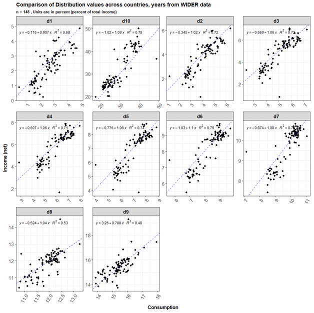
Figure 3 Consumption distribution deciles (x axis) compared to net income distribution deciles (y axis) across all country-year observations. Dashed lines show the 1:1 linear relationship. The solid line is the used regression line. Only observations for half the dataset are selected (pre-2004) for the plot.

Consumption distribution deciles are converted into net income deciles using Eq. (1) (which was fit using a linear regression for each decile) below:

$$\begin{array}{}\text{(1)}& D_{{\text{netincome}}_{n,r,t}}=a_n\cdot D_{{\text{consumption}}_{n,r,t}}+b_n,\end{array}$$

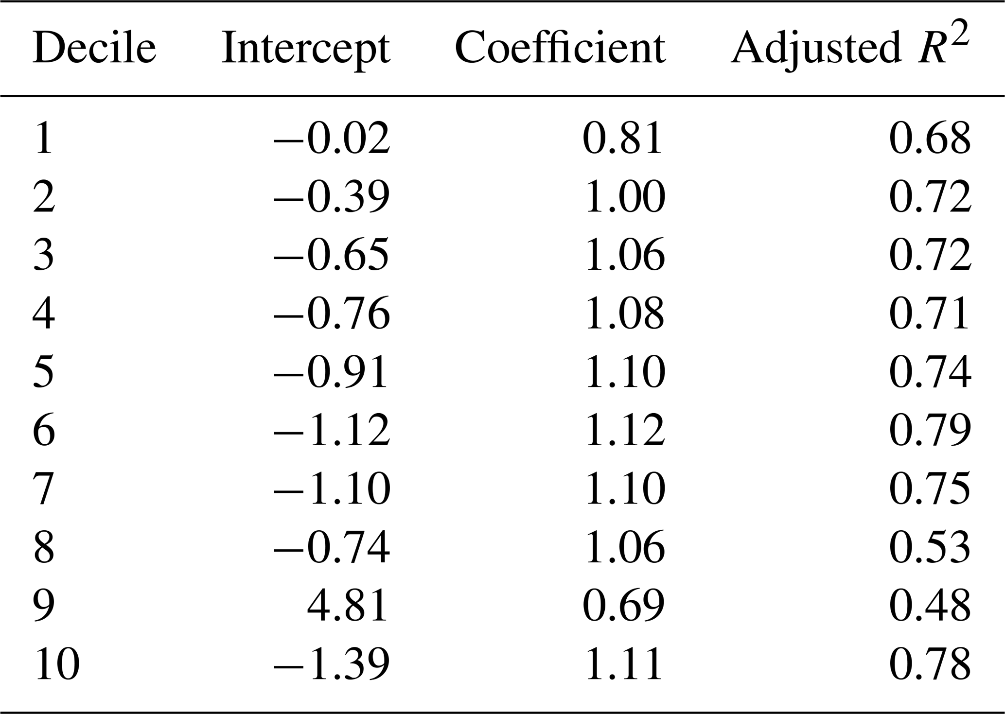
where D is the share of consumption or income in a particular decile between 0 and 100, and a is the coefficient applied to each decile parameterized using a linear regression documented in Table 4. b is derived from linear regressions run for each decile documented in Table 4, n is the decile ranging from 1 to 10, and r and t are the region and time step, respectively.

Table 4 Summary of the coefficients and intercepts by decile used by Eq. (1). These are fit based on 148 data points.

2.3.1 Validation of our approach

We then verified the performance of our regression on a testing dataset (Fig. 4). We note that the R² values in our testing dataset are similar to those in our training dataset, and we also note that the imputed values are within a 5 % confidence interval of actual values. To validate our imputation method, we calculated errors (imputed shares − actual shares) for our testing dataset (n=109). We compared the error by decile for the dataset (see Fig. S1 in the Supplement). The mean error across deciles is generally within 0.5 % across all the years. There are larger differences for the year 2011, where we had very few observations. We have also verified that all the imputed decile values add up to 1.

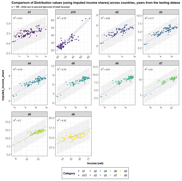
Figure 4 Comparison of actual and imputed values in our testing dataset. Different deciles are shown as facets, and we also show the confidence interval. All the imputed values are found to be within a 5 % confidence interval of the original values.

We note that this imputation method is applied to a small subset of observations (394) out of the total number of observations in our dataset (8522). We also acknowledge that this method is simple and should be improved upon in future updates and analyses.

2.4 Imputing net income deciles based on summary measures of the Gini coefficient

As observed in Table 1, the majority of the observations in our dataset are those from the imputation from the Gini coefficient. In this section we will explain this imputation approach, i.e., why a new imputation approach was necessary and why this approach is an improvement upon existing methods.

For many country years, no data are available for the income or consumption deciles based on household survey data. However, the World Development Indicators (WDI) dataset (Reid, 2012) does provide aggregate measures of income distribution, such as the Gini coefficient for some country-year observations.¹ Many studies have utilized the Gini coefficient in combination with different functional forms to estimate the underlying income distribution (Shorrocks and Wan, 2008; Soergel et al., 2021). Most prominent amongst these methods is the usage of the lognormal functional form along with the Gini coefficient to derive the underlying distribution.

However, methods such as the lognormal functional form have documented limitations. For example, the observations are known to deviate from lognormal in the tails of the distribution (Badel et al., 2020; Chotikapanich, 2008). Moreover, the lognormal functional form is assumed for every country for every year. Recently, a nonparametric approach was developed which uses the Gini coefficient in combination with a two-component model based on a PCA to produce a more accurate estimate of income deciles (Narayan et al., 2023). This method addresses some of the limitations of the lognormal functional form. The performance of the nonparametric PCA-based approach compared to the lognormal functional form is described in more detail in Fig. 5 below. We found that the PCA-based approach improves the fit across several deciles compared to the lognormal functional form. The paper by Narayan et al. (2023) contains a more extensive discussion of the model fit and comparisons of fit across countries, years and individual deciles. Given that the method provided a good fit to the historical data on income distributions, we use this method to impute income deciles where only the Gini coefficient is available.

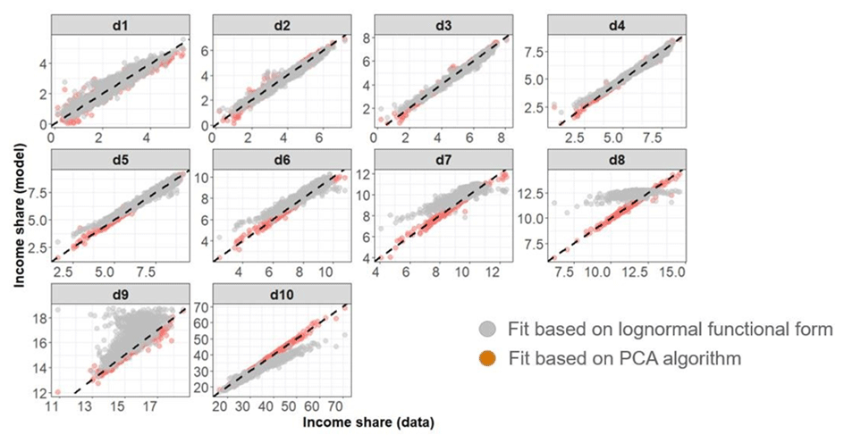
Figure 5 Comparison of fits of lognormal functional forms (grey dots) with PCA-based fits (orange dots) with data for each decile (facet). The lines represent the 1:1 fit between the x and y axes. Income shares are expressed as a percent of the total income.

For country years where we could not find data on net income or consumption, we used this PCA-based approach along with observed values of the Gini coefficient from the World Development Indicators Database (Reid, 2012) to impute the underlying net income distribution.

The PCA-based approach can be described as follows.

The income deciles are calculated as

$$\begin{array}{}\text{(2)}& D_{r,t}=a_{r,t}\mathrm{PC}\mathrm{1}+b_{r,t}\mathrm{PC}\mathrm{2},\end{array}$$

where D is a 10-dimensional vector of income shares for all the population deciles in region r at time t. PC1 and PC2 are the two principal components, which are also vectors of length 10 (the values of PC1 and PC2 are provided in Fig. S2 and Table S3). a and b are coefficients of the two principal components specific to each region and time.

The coefficient a is derived from the Gini coefficient using a regression equation estimated on 1659 observations of national net income distribution:

$$\begin{array}{}\text{(3)}& a_{r,t}=-\mathrm{11.4815}+\mathrm{29.71708}\cdot {\mathrm{Gini}}_{r,t}.\end{array}$$

The coefficient b is estimated using lagged values of the Palma ratio ($d\mathrm{10}/(d\mathrm{1}+d\mathrm{2}+d\mathrm{3}+d\mathrm{4})$), the income share in the ninth decile and the current period labor share of the GDP (gross domestic product):

$$\begin{array}{}\text{(4)}& \begin{array}{rl}{b}_{r,t}& =-\mathrm{17.18222}+\left(\mathrm{1.07957}\cdot {\mathrm{LabShareGDP}}_{r,t}\right)\\ & +\left(\mathrm{113.10810}\cdot {\text{ninth\hspace{0.17em} decile}}_{t-\mathrm{1}}\right)\\ & +\left(-\mathrm{0.36392}\cdot {\text{Palma ratio}}_{r,t-\mathrm{1}}\right).\end{array}\end{array}$$

Using this approach, we were able to fill in values for various country years. The observations in our dataset are summarized in Table 1 above.

As mentioned and discussed above, the PC algorithm used for the imputation was tested against the latest data on decile-level income distributions and provided a good fit for all deciles across all countries. This testing was performed for both in-sample and out-of-sample observations. This PCA-based method was also found to yield a better fit to the data when compared to other methods, such as using the Gini coefficient in combination with a lognormal functional form.

Since we used a summary measure (the Gini coefficient) to derive the underlying distribution, we also validated our imputation approach by recalculating the Gini coefficient from the imputed distribution and comparing it with the reported Gini coefficient (Fig. 6). We observe that our recalculated values largely have a 1:1 correlation with the input Gini values, suggesting that the imputation did not introduce many errors (the overall R² value of the comparison is 0.99). However, the relationship does start to weaken for countries with very high Gini coefficients, such as South Africa, where the recalculated Gini coefficient is different from the observed Gini coefficient by as much as 0.07 points. This is a result of the parameters of the PCA algorithm, which do not reproduce values well for outlier countries with extreme Gini coefficients. We also observe that the recalculated Gini coefficients for some countries are different in different years. For example, in Malawi, there are large year-to-year jumps in the reported Gini coefficients from year to year (Fig. S3).

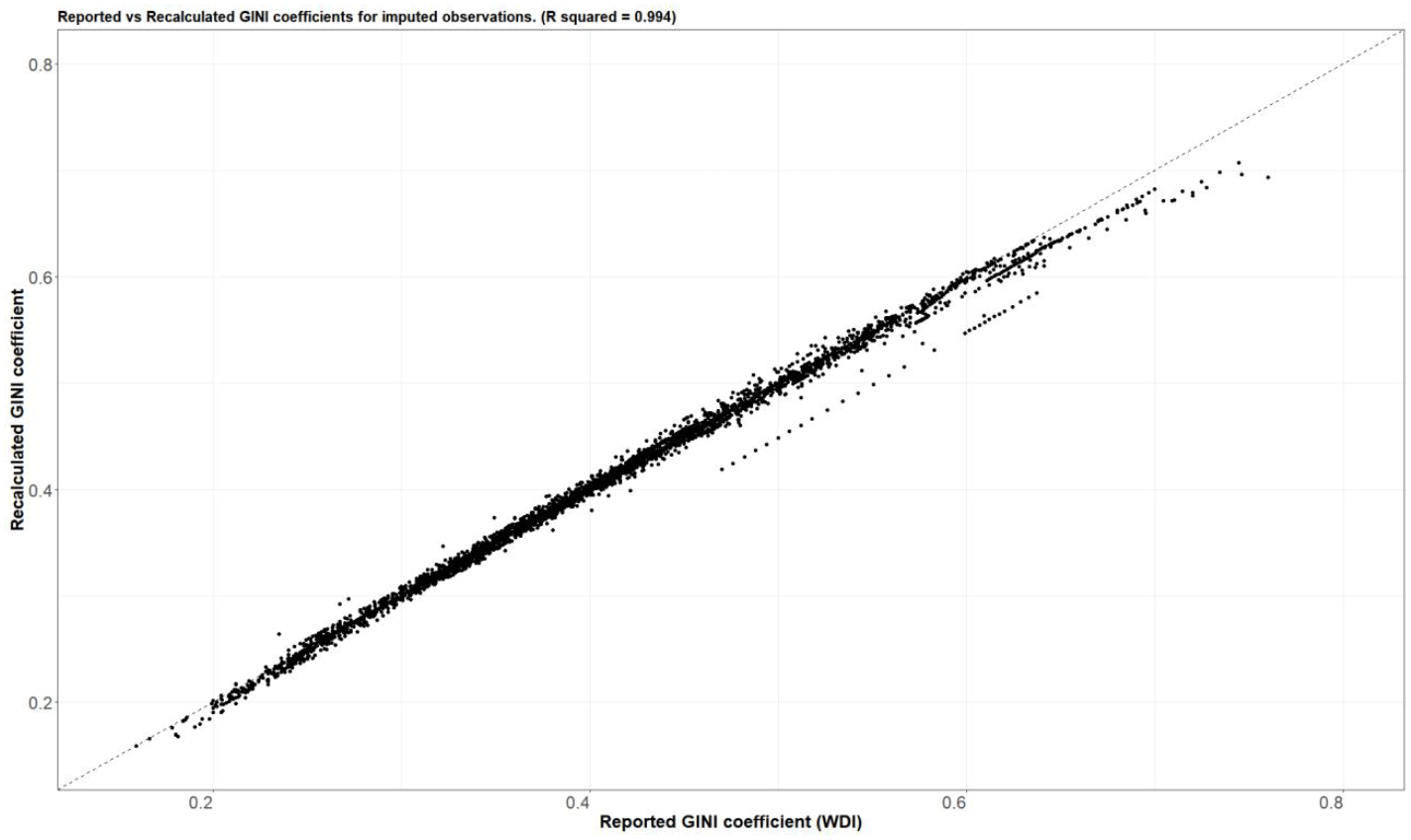
Figure 6 Comparison of the reported Gini coefficients from the WDI (x axis) with the recalculated Gini coefficients from the imputed distribution (y axis). Each dot is a country-year observation. The dashed line represents a 1:1 relationship.

We also evaluated temporal trends in the complete dataset, which now include values from direct observations and also imputed values. The top two panels in Fig. 7 below show trends in the income shares for the 10th decile for India and China across time from all data sources.

This approach helps us generate better coverage in our dataset, and the PCA model provides a statistically valid method for generating the data from Gini coefficients. This approach does have some limitations, however. The Gini coefficients from the WDI can represent multiple income concepts. For example, in the US, the Gini coefficient from the World Development Indicators Database is based on gross income, and the income distribution based on surveys (from the LIS) is for net income; i.e., it includes adjustments for direct taxation.² Moreover, it is unclear when the Gini coefficients are based on simple interpolation or on country-level or subnational survey data. This further makes it important to clearly understand and document the source of the Gini coefficients used.

As a first step in addressing this, we used data from the “All the GINIs” dataset, which clearly specifies the income concept of the derived Gini coefficient (G. Ferreira et al., 2015; Smeeding and Latner, 2015), to identify the income concepts of the Gini coefficients used for interpolation. Based on that, we identified that roughly 4200 observations of the Gini coefficients used for imputation are net income Gini coefficients, while the rest are consumption or expenditure Gini coefficients or gross income Gini coefficients (Table 5). Therefore, data points when derived from imputation of a consumption, expenditure or gross income Gini coefficient have been marked as such in our final dataset. Users can choose to use all data points together or filter data depending upon their needs.

Table 5 Descriptions of the sources of the Gini coefficients used for imputation.

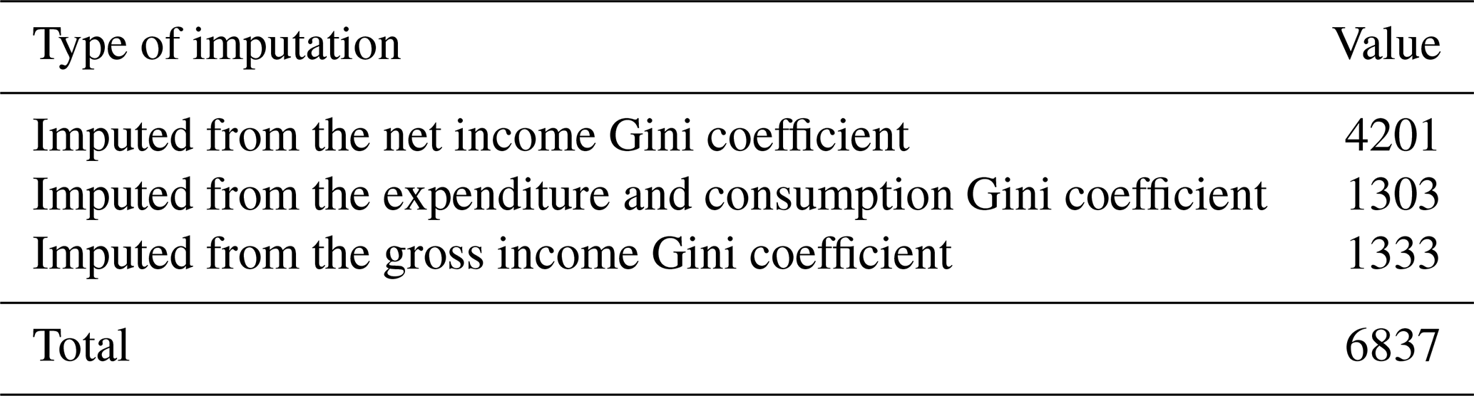
Given that the “All the GINIs” dataset still offers only a limited time series, this still suggests a limitation in our imputation approach, and one possible next step would be to only use net income Gini coefficients for the imputation of the decile-level income distribution. Figure 7 below shows the full time series of our dataset (for the 10th decile) based on different types of imputation performed.

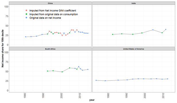
Figure 7 Temporal trends in the 10th decile for the complete dataset. Colors represent different data sources.

3 Aggregating income distributions to the regional level

The motivation for developing this country-level dataset was to initialize decile-level income distribution values for GCAM. Models like GCAM operate on regional boundaries and therefore would require the income distributions to be aggregated to their respective regional boundary conditions. We aggregated the income distributions from the country level to 32 geographic regions represented by GCAM. The 32 regions are shown as a map in Fig. 8.

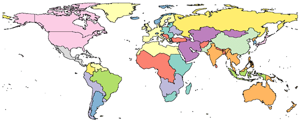
Figure 8 Map of the 32 GCAM regions. These 32 GCAM regions are based on 229 country boundaries.

Aggregating income distributions to the regional (where a region is made up of multiple countries) level is not straightforward because countries within regions differ in population size, average income level and level of inequality in the income distribution. For example, an individual who belongs to the 10th decile in Romania would not necessarily be counted amongst the 10th decile of Europe as a whole, given the difference in the overall income level of Romania relative to the higher income levels of other European countries such as Germany and France. Similarly, even countries with similar average income levels may differ significantly in how income is distributed across deciles.

The aggregation of the country-level income distributions to the regional income distributions involved the following steps.

1. First, we sorted all country net income deciles in the region by the average decile income level, from lowest to highest income (the net income distribution shares are applied to this GDP per capita, measured in PPP (USD 2011) to arrive at the income level). We use GDP per capita here, since that variable is the income proxy in GCAM.

2. Next, we calculated the cumulative population for each of these country income groups. The cumulative population over all the country income groups matches the regional total population.

3. We then calculated cumulative population cutoffs that would create regional population deciles by dividing the regional population by 10.

4. Based on these cutoffs, we calculated the regional decile shares of income by assuming a uniform distribution of income within each country decile. Thus, wherever a country decile spanned a regional cutoff, its income was split between regional deciles in proportion to the country population falling in each regional decile.

Figure 9 below illustrates our aggregation approach for GCAM region 14, Europe Non-EU, which is made up of Albania, Bosnia, Croatia, Macedonia, Montenegro, Serbia and Türkiye. The figure demonstrates that a given regional decile can contain a mix of deciles at the country level. For example, the regional d2 consists of d3 and d4 values of some low-income countries such as Serbia and Albania. The regional d10 contains both the d9 and d10 values from Türkiye.

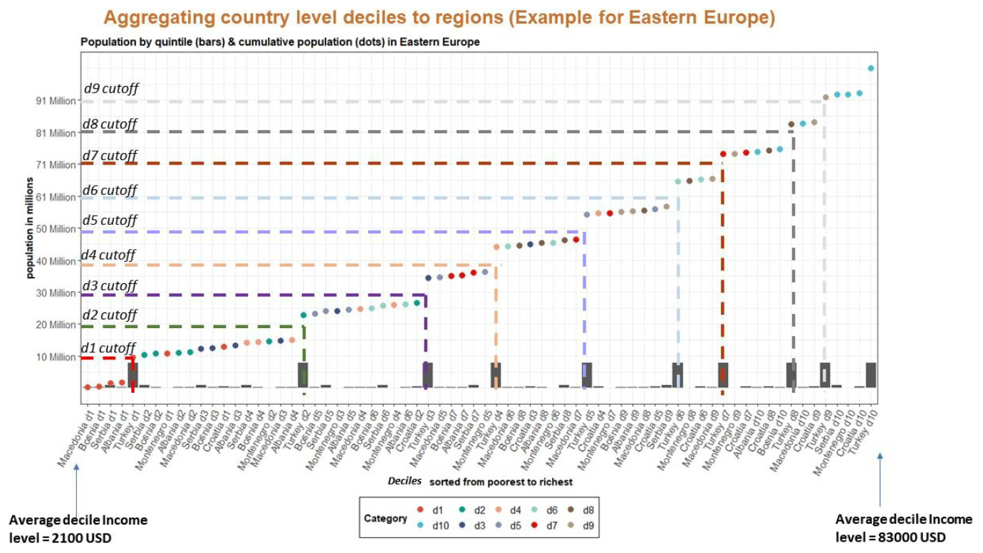
Figure 9 Explanation of our aggregation approach. On the x axis, all deciles within the region are sorted from low income to high income. Bars track the population. The dots show the cumulative population compared to the decile-level income. The dashed lines show the new regional cutoffs for the deciles.

We also compared the aggregated income distribution to the country-level income distributions for 2015 (Fig. 10). We find that the aggregated income distributions are mostly driven by trends in the income distribution of the most populous countries in the region, as expected. In the example above, the income distribution for GCAM region 14 (Europe Non-EU) is largely driven by the income distribution of Türkiye, which is the most populous, and most unequal, country in that region (e.g., Türkiye represents approximately 75 % of the regional population in 2015). There are certain cases where the regional distribution is significantly different than the country-level distribution. In central Asia, for example, the regional income distribution is much more unequal (the regional Gini coefficient is 0.53) compared to the country-level Gini coefficients (the highest Gini coefficient is 0.39). This is because there is considerable variation in the income levels across the countries. The country-level average incomes range from USD 2011 in Tajikistan to USD 23 485 in Uzbekistan. This further illustrates why a specific aggregation method was necessary to construct these regional income distributions (simple aggregation methods would miss such intra-regional dynamics).

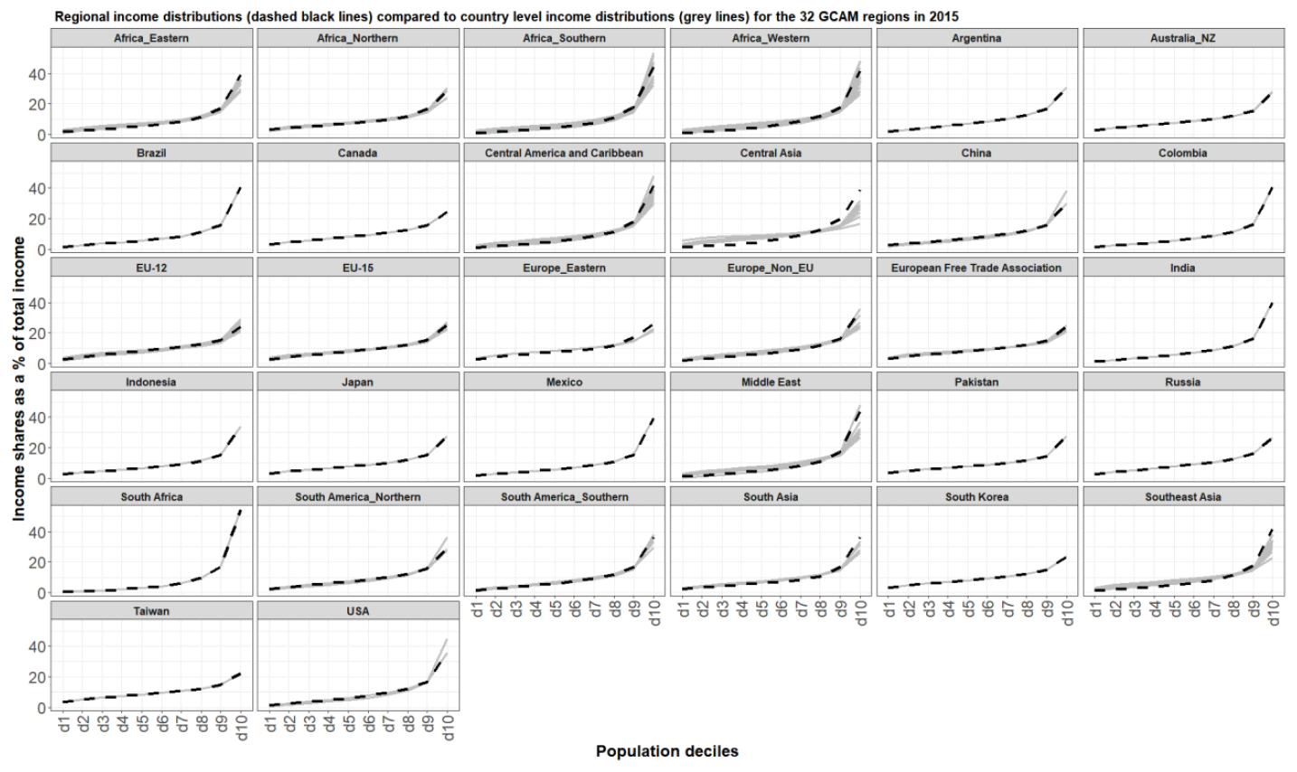
Figure 10 Regional income distributions (dashed black line) compared to the national income distributions (grey lines) in each of the 32 regions in 2015.

Table 6 Coverage by data status in terms of GDP in PPP and population from the Shared Socioeconomic Pathway (SSP) database V9.

4 Quantifying coverage and assessing regional bias in the data

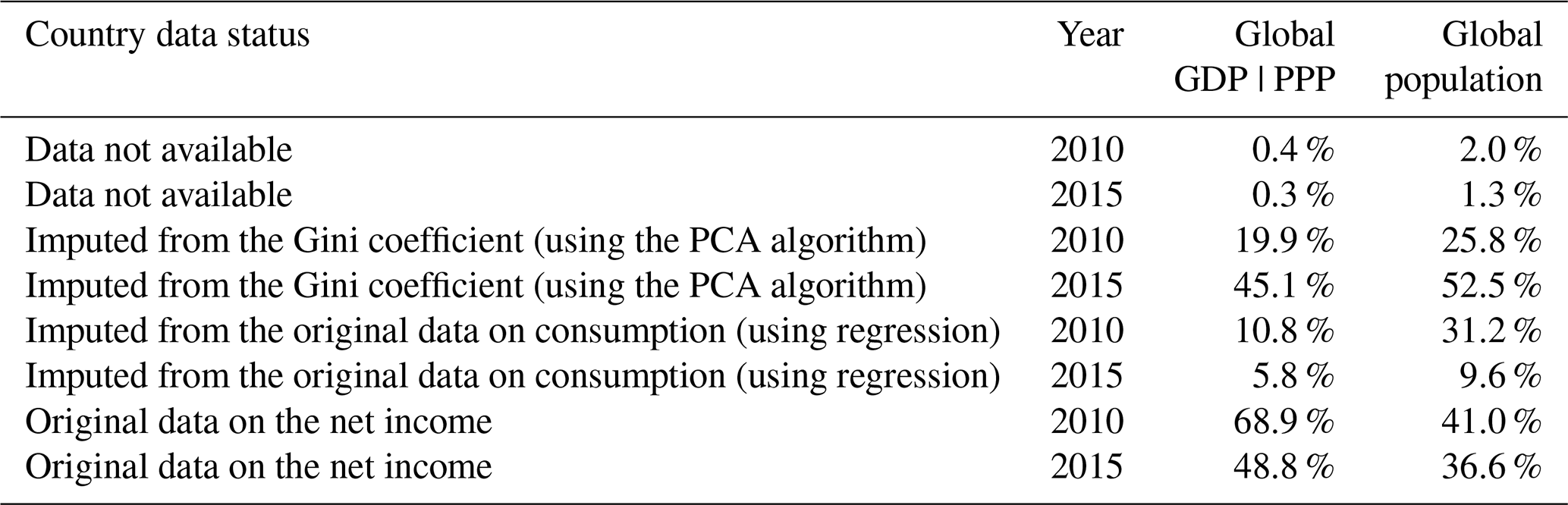
As mentioned earlier, we intended to develop a dataset for net income distribution for the 229 countries aggregated to 32 regions used in GCAM. As shown in Table 5, we were unable to find any data on net income or consumption for 39 of those 229 countries. Previous models that have been developed for projecting income distributions have been based largely on data for high-income countries (Rao et al., 2019; Pachauri, 2020).

In order to evaluate whether the lack of data for the 56 countries introduces a bias, we assessed the data coverage in terms of percent of global population (total population of 229 countries) and percent of global GDP (total GDP at MER (market exchange rate) for 229 countries) for our dataset. We found that our dataset covers 98 % of the global population and 93 % of the global GDP in any given year.

Similarly, we also compared the population and GDP of countries with and without data for 2 years (Table 6) and found that the countries that are missing data in the latest historical year (2015) only constitute 1.3 % of the global population and 0.3 % of the global GDP. The biggest countries that are missing data in terms of population in 2015 are Morocco (33 million people), North Korea (24 million people) and Somalia (10 million people). In terms of GDP, the biggest countries missing are Morocco (USD 123 billion at PPP), Oman (USD 68 billion at PPP) and Equatorial Guinea (USD 18 billion at PPP).

Further, Fig. 11 below shows the data availability status (from Table 6) as a map to show the status of data availability by ISO code.

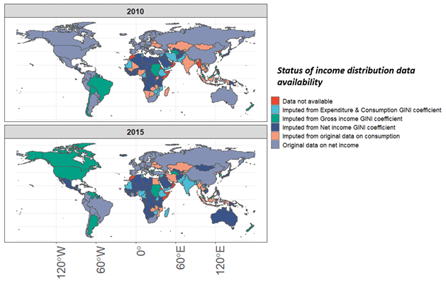
Figure 11 Data availability by country. The availability is shown here for the two years 2010 and 2015.

Since these data will be used to initialize income distributions in GCAM, we also evaluated whether the data would introduce a bias for any GCAM region (e.g., whether is there no coverage or poor data coverage for any given GCAM region).

To evaluate this, we divided the countries in our dataset into the 32 geographical regions modeled by GCAM. We then assessed the data coverage in terms of a percent of population (Table S4) and GDP (Table S5) for each of these regions. While these regions are specific to a particular model, they also represent heterogeneity across countries well in terms of regional economic and demographic conditions.

An example of a result of this assessment is that in the region of eastern Africa we found data that cover 64 % of the region's population in 2010 and 40 % of the region's GDP for the same year. We performed this assessment for 5 years from 2010 to 2015. The purpose of this assessment is to verify whether we have some coverage of data for all regions of the world within those 5 years, which would increase our confidence that our models are not biased towards high-income countries. The lowest coverage in our dataset is found for the Middle East region, where our data cover roughly 60 % of the region's population and 40 % of the region's GDP.

5 Updating data in the future

As noted in the sections above, our dataset currently contains data for the national income distribution from 1958 to 2015. This is largely because these data were produced to calibrate GCAM, whose final model base year is 2015. We will update this dataset to the most recent years in the near future. Users interested in extending the dataset by themselves can make use of the R scripts made available as part of the pridr software package (available here – https://github.com/JGCRI/pridr, last access: 7 May 2024) to perform the extension.

6 Data availability

The main dataset is available here on Zenodo (https://doi.org/10.5281/zenodo.7093997) (Narayan et al., 2022b). There are two main datasets available:

1. 32 regional income deciles from 1958 to 2015 and

2. ISO-level income distributions from 1958 to 2015.

Note that the income distribution data can be flexibly generated using the pridr software package available on Zenodo (https://doi.org/10.5281/zenodo.7468250, Narayan et al., 2022a).

7 Discussion

In this paper we present a new consistent dataset on the net income distribution across 190 countries from 1958 to 2015. This dataset is also available for 32 aggregated regions. To our knowledge there is no other dataset that presents consistent data at multiple geographical scales that have been documented in a peer-reviewed article. This complete and harmonized dataset may be useful for efforts related to t modeling of the net income distribution.

The aggregation method presented in this paper (Sect. 3) takes into account both within-country and across-country inequality when aggregating income distributions to regional boundaries. This is important to regions where there is significant diversity in the income distribution across regions such as central Asia, where the aggregated income distribution is significantly more unequal than in any of the member countries (Fig. 10).

There are a number of areas of improvement that we have noted that can be explored as next steps or in future updates to this dataset. First, we have used a simple linear regression approach when converting the consumption distributions to the net income distribution. This can be improved upon if more data become available (related to the savings rate across countries) or if the income within countries can be broken down into the various incomes and expenditures, similarly to a computable general equilibrium (CGE) framework.

Similarly, while our imputation approach greatly increased spatiotemporal coverage in our dataset, we noticed that the Gini values from the WDI can represent multiple income concepts. In the future, these gross income or consumption Gini coefficients should also be converted to net income Gini coefficients before the imputation. This would require more detailed data on the input Gini coefficients. One possible next step would be to construct a method for such a conversion using Gini values from datasets such as the “All the GINIs” dataset, which tracks the type of Gini coefficient (G. Ferreira et al., 2015; Smeeding and Latner, 2015). Another option would be to explicitly generate a tax adjustment to convert gross income values to net income.

We further note that we utilized a single equivalence scale to represent our income distributions (per capita). However, we have not tested the effect of changing equivalence scales on income distributions. This can be tested in the future.

We further found that the PCA-based imputation approach underestimates inequality when imputing the income distributions of highly unequal countries such as South Africa. As more data on income distributions become available, the PCA algorithm can be re-parameterized to newer data. When this happens, the imputation should be re-performed.

Finally, the data generation described above is documented as an open-source workflow of a software package called pridr, which can be used to generate and re-aggregate these data. The software package is available on GitHub, and the dataset itself is available as a version-controlled release on Zenodo (see the Data availability section).