the Creative Commons Attribution 4.0 License.
the Creative Commons Attribution 4.0 License.
 | 26 May 2021
Comprehensive bathymetry and intertidal topography of the Amazon estuary
Alice César Fassoni-Andrade
Fabien Durand
Daniel Moreira
Alberto Azevedo
Valdenira Ferreira dos Santos
Claudia Funi
Alain Laraque
The characterization of estuarine hydrodynamics primarily depends on knowledge of the bathymetry and topography. Here, we present the first comprehensive, high-resolution dataset of the topography and bathymetry of the Amazon River estuary, the world's largest estuary. Our product is based on an innovative approach combining spaceborne remote sensing data, an extensive and processed river depth dataset, and auxiliary data. Our goal with this mapping is to promote the database usage in studies that require this information, such as hydrodynamic modeling or geomorphological assessments. Our twofold approach considered 500 000 sounding points digitized from 19 nautical charts for bathymetry estimation, in conjunction with a state-of-the-art topographic dataset based on remote sensing, encompassing intertidal flats, riverbanks, and adjacent floodplains. Finally, our estimate can be accessed in a unified 30 m resolution regular grid referenced to the Earth Gravitational Model 2008 (EGM08), complemented both landward and seaward by land (Multi-Error-Removed Improved-Terrain digital elevation model, MERIT DEM) and ocean (General Bathymetric Chart of the Oceans version 2020, GEBCO_2020) topographic data. Extensive validation against independent and spatially distributed data, from an airborne lidar survey, from ICESat-2 altimetric satellite data, and from various in situ surveys, shows a typical vertical accuracy of 7.2 m (riverbed) and 1.2 m (non-vegetated intertidal floodplains). The dataset is available at https://doi.org/10.17632/3g6b5ynrdb.2 (Fassoni-Andrade et al., 2021).
- Article
(11923 KB) - Full-text XML
- BibTeX
- EndNote


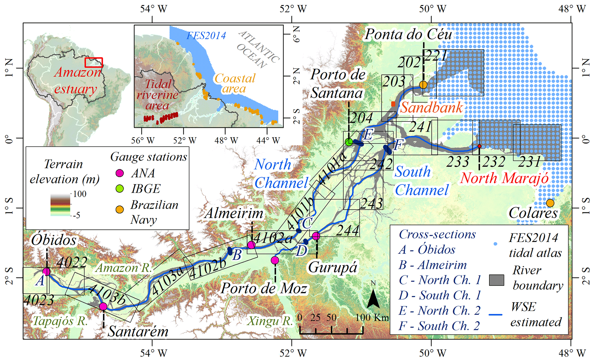
Figure 1Location of the Amazon River estuary, identifying and delimiting nautical charts (Brazilian Navy – black boxes) and showing the locations of gauge stations of the Agência Nacional de Águas (ANA), the Brazilian Navy, and the Instituto Brasileiro de Geografia e Estatística (IBGE). Terrain elevation from MERIT DEM.
The Amazon River exports the largest discharge of freshwater (205 000 m3 s−1; Callède et al., 2010) and the largest sedimentary supply (5–13×108 t yr−1; Filizola et al., 2011) worldwide. However, to date, no consistent, comprehensive, publicly available topographic dataset has been available for the estuary that can support hydrodynamic, sedimentary, or ecological studies. The largest estuary in the world is home to energetic exchanges of momentum between the upstream river and the ocean, with a marked variability in the water level over a broad range of timescales, from the semidiurnal tide propagating upstream from the Atlantic Ocean to the interannual hydrometeorological climatic events frequently occurring over the upstream catchment. These exchanges between the river and the ocean result in sporadic flooding events, which profoundly impact the riparian communities' socioeconomic conditions (Andrade and Szlafsztein, 2018; Mansur et al., 2016). The morphology of the riverbed is known to primarily condition the estuary's hydrodynamics, particularly the propagation of the tidal wave (Gallo and Vinzon, 2015), which is expected to affect the dynamics of the riverine floods and the extent of the associated flooding (Kosuth et al., 2009). This dynamic environment with high ecological diversity is essential for nutrient cycling and carbon fluxes (Sawakuchi et al., 2017; Ward et al., 2015), for navigation (Fernandes et al., 2007), and for the transport and accumulation of sediment (Nittrouer et al., 2021).
The Amazon estuary extends from the continental shelf up to Óbidos city, corresponding to the longest tidally influenced reach in the world, extending over 800–910 km (Kosuth et al., 2009; Nittrouer et al., 2021; Fig. 1). This river flow is drained downstream towards the ocean through the main channel until the confluence with the Xingu River, around 300 km upstream of the mouth, where it is divided into two long channels, hereafter called “South Channel” (locally named Gurupá Channel) and “North Channel” (Fig. 1). Downstream of this branching, the estuary appears as a complex network of dendritic tidal channels and islands (Fricke et al., 2019). The estuary is classified as macrotidal (Dyer, 1997; Gallo and Vinzon, 2005) and semidiurnal (Kosuth et al., 2009) with a tidal range between 4 and 6 m at the mouth. The M2 (lunar semidiurnal) and S2 (solar semidiurnal) tidal constituents are the dominant components at the ocean boundary, with respective amplitudes of 1.5 and 0.4 m there (Gallo and Vinzon, 2005). At the upstream limit of the estuary in Óbidos, the range of the drought–flood annual cycle of the river height typically amounts to 6 m, and the tidal effects remain detectable only during the drought season (Kosuth et al., 2009). Thus far, the quantitative investigation of the estuary's hydrodynamics and the interaction mechanisms between the tide and the river flow has been limited by the lack of sufficiently resolved bathymetric databases (e.g., Gabioux et al., 2005). Therefore, past hydrodynamical studies of the Amazon estuary relied on approaches based on box models (Prestes et al., 2020) and/or on coarse hydrodynamical models (e.g., Gallo and Vinzon, 2015). Still, these past studies revealed rich hydrodynamics of the estuary, comprising contrasting patterns of bottom friction (Gabioux et al., 2005), active nonlinear deformation of the tidal waves (Gallo and Vinzon, 2005), a distinct structure of the salinity front (Molinas et al., 2014, 2020), and a prominent role of the intertidal flats in the flow variability (Gallo and Vinzon, 2005). The interplay between the fluvial variability in the water level and its tidal variability is particularly known to exert a central control on the estuary's sedimentation pattern (Fricke et al., 2019). While the geometry of the Amazon estuary is known to have been influenced little by anthropogenic effects to date, it appears essential to document it in its current state, at a time when the human influence is rising and is expected to induce profound, long-lasting impacts on the continental sediment supply to this estuary (Latrubesse et al., 2017).
The present paper aims to present a novel topographic and bathymetric dataset of the whole Amazon River estuary, from its upstream limit 1000 km inland to its terminal estuary at its oceanic outlet, covering the riverbed as well as the intermittently flooded riverbanks and adjoining floodplains. Over the continually wet part of the riverbed, we rely on a traditional methodology to construct the bathymetry based on comprehensive, systematic digitization of existing nautical charts. In contrast over the intermittently dry intertidal zones and floodplains, our mapping is achieved through an original, state-of-the-art approach based on spaceborne remote sensing. Our dataset is regularly gridded at a 30 m resolution and elevations are referenced to the Earth Gravitational Model 2008 (EGM08; Pavlis et al., 2012). It covers the river streams, riverbanks, and floodplains, and it extends downstream of the estuary mouths over the near-shore ocean shelf and open-ocean coastline, covering the domain shown in Fig. 1.
The remainder of the paper is structured as follows: Sect. 2 presents the data sources and the methods used to build the dataset; Sect. 3 presents the validation against independent databases; Sect. 4 shows the topographic mapping and cross section along the river and floodplain; Sect. 5 discusses the significance and caveats of the dataset; and Sect. 6 explains the access to the various forms of our dataset.
2.1 Bathymetry of the riverbed
Over the continually wet part of the various streams of the Amazon estuary, the approach relies on systematic digitization of sounding points of bed elevation harvested from a comprehensive ensemble of nautical charts published by the Brazilian Navy (available at https://www.marinha.mil.br/chm/dados-do-segnav/cartas-raster, last access: 29 July 2020). Although technically straightforward, this task was by far the most tedious part of the procedure, on account of the large geographical extent of the domain (21 500 km2, gray polygon in Fig. 1). We digitized more than 500 000 individual points from a total of 19 charts, which are identified and delimited in Fig. 1. The primary bathymetric surveys utilized in these charts were carried out by the Brazilian Navy on different dates varying between 1953 and 2019, with a reasonably large fraction of them done after 2000 (see Table A1 for further details). Figure 2a displays an example of a digitized nautical chart. One issue with the maps that we could access was the vertical referencing of the digitized elevations. Depending on the map considered, the bed elevation values were provided with respect to two different reference water surface elevations (WSEs): either the level of the 90th percentile of water surface elevation (hereafter referred to as WS90) or the average level of the low tide during the spring tide (termed syzygy and hereafter referred to as SYZ).
We inferred the vertical elevation of each of these two references from the available records of the tide gauge stations scattered along the river down to the river mouth. The tidal and limnigraphic records from the seven stations that we could access, listed in Tables A2 and A3 (locations in Fig. 1), were provided by the Agência Nacional de Águas (ANA), the Brazilian Navy, and the Instituto Brasileiro de Geografia e Estatística (IBGE). The vertical water level of both references (WS90 and SYZ) was deducted explicitly from the temporal records by computing the level of the 90th percentile to infer WS90 and by computing the average level of the low tide during spring tides for SYZ. These references were computed with respect to the geoid considering the absolute leveling published in Calmant et al. (2013) and Callède et al. (2013), complemented by a dedicated geodetic field survey that we conducted in January–February 2020 (Appendix A). At the river mouth, downstream of the downstream-most tidal stations (blue points in Fig. 1), the SYZ level was calculated using a combination of the mean sea surface height provided by the ocean general circulation model of Ruault et al. (2020) and of a proxy of the syzygy level estimated by the FES2014 tidal atlas (Carrère et al., 2016; available at https://www.aviso.altimetry.fr/en/data/products/auxiliary-products/global-tide-fes.html, last access: 1 November 2020). This proxy for SYZ was defined classically according to Eq. (1), from the sum of the amplitudes of the M2 and S2 tidal constituents (Pugh and Woodworth, 2014):
We inferred the WSE (i.e., WS90 or SYZ, depending on the reference of the chart under consideration) separately along the Amazon River (Óbidos, Santarém, and Almeirim), the North Channel (Porto de Santana and Ponta do Céu), and the South Channel (Almeirim, Porto de Moz, Gurupá, and a point of the FES2014 tidal model marked as “North Marajó” in Fig. 1) via linear interpolation between the successive stations, resulting in the profile shown in Fig. 2c. The linear interpolation considered successive points along the river spaced by 30 m and represented by the two blue lines in Fig. 1. The WSE for each of the 500 000 digitized points was then inferred from the values along the river via a nearest-neighbor interpolation method. Following this, the WSE was subtracted from the water depths, resulting in bed elevation values referenced to EGM08. The bed elevation points were then interpolated using the “topo-to-raster” method (Hutchinson, 1989), which is essentially an interpolation method suited to hydrological objects to create a regular elevation grid with a 30 m spatial resolution.
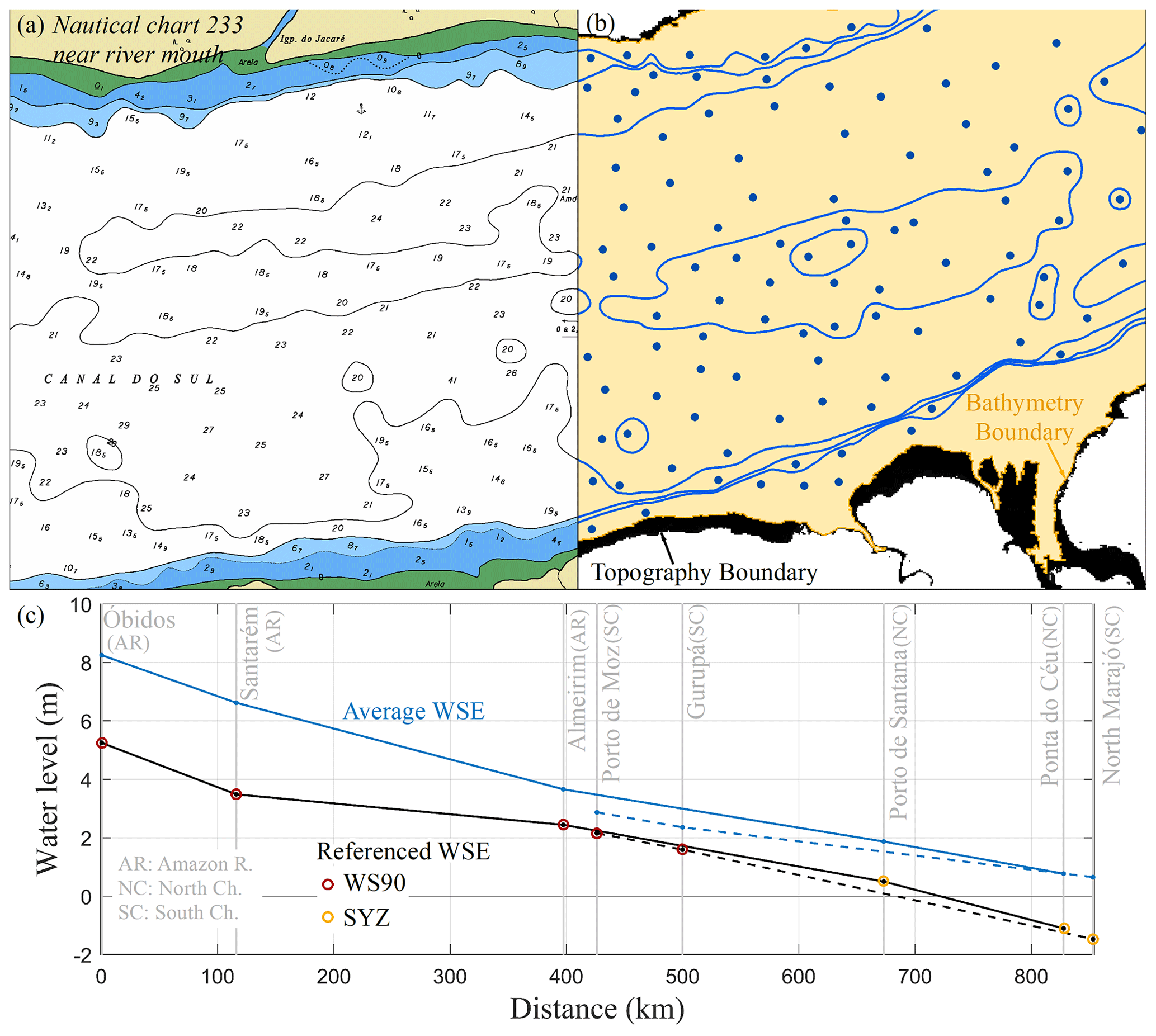
Figure 2(a) Example of a nautical chart near the river mouth (code 233). (b) Digitized pointwise soundings and isobaths, along with bathymetric boundaries (defined as the 96 % isoline of flood frequency) and topographic boundaries (defined as the 0 % isoline of flood frequency); the two regions are immediately adjacent. (c) Referenced WSE (black lines) and average WSE (blue lines) along the Amazon estuary (EGM08 geoid).
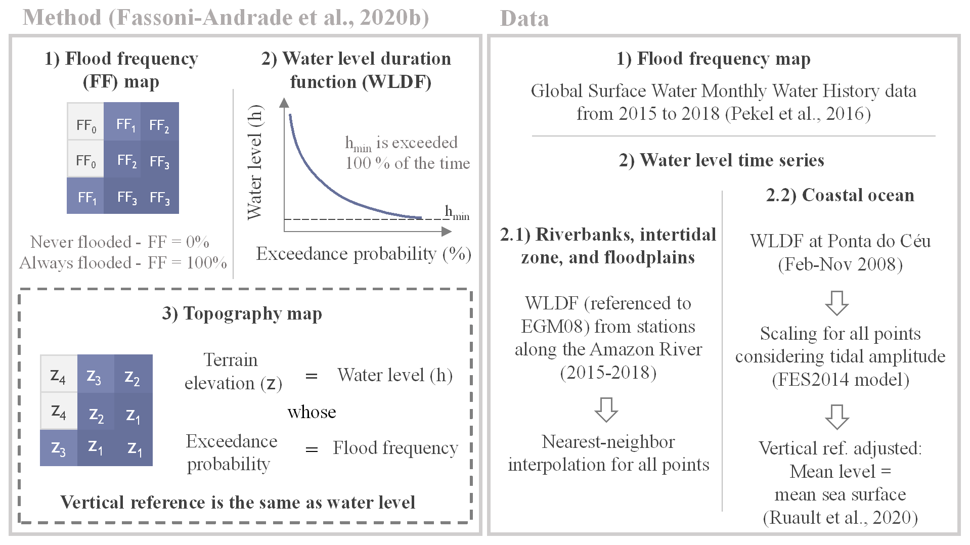
Figure 3Method to estimate the topography of the water bodies (Fassoni-Andrade et al., 2020b; left panel) and the various datasets considered in this study to implement this method (right panel).
In the interpolation, a river boundary was considered, as shown in Fig. 1 (gray polygon) and exemplified in Fig. 2b (bathymetric boundary). This boundary is a polygon defined considering a flood frequency of between 96 % and 100 %. The flood frequency map was calculated from the Global Surface Water (GSW) Monthly Water History v1.2 data (Pekel et al., 2016; available at https://global-surface-water.appspot.com, last access: 3 August 2020), which represents the spaceborne Landsat-based monthly record of water presence on a global scale with a spatial resolution of 30 m. A Google Earth engine code (Gorelick et al., 2017), described in Fassoni-Andrade et al. (2020b), was used to create the flood frequency map and considered all GSW monthly images from the period from January 2015 to December 2018, resulting in a total of 48 months. This 48-month period was found to be a good compromise between a short enough period to ensure that the dataset was recent enough and a long enough period that it was capable of capturing the bulk of the flooding statistics.
2.2 Topography of periodically flooded areas
Intertidal banks and floodplains are areas periodically flooded by tides and riverine floods, respectively. We define them as the areas comprising between 0 % and 96 % of the abovementioned flood frequency map. In past studies devoted to coastal mapping, intertidal topography has been mapped using remote sensing data, with the waterline method being one of the most widely adopted techniques (see Salameh et al., 2019, for a review). This method requires the detection and extraction of the water contours in imagery time series. Next, water levels are assigned to the individual water contours, creating isobaths. A digital elevation model (DEM) raster can be generated from a large enough amount of such isobaths. Some recent applications of this method are found in Bell et al. (2016), Bergmann et al. (2018), Bishop-Taylor et al. (2019), Khan et al. (2019), and Salameh et al. (2020). This method has proven tractable with moderate-resolution spaceborne imagery; however, it requires simultaneous water level knowledge at the exact time of each acquisition, along the remotely sensed waterlines. It also relies on spatial interpolation of the isobaths between successive waterlines, which can be problematic if the waterlines are sparse. Recently, alternative methods have been developed using a flood frequency map to estimate the coastal topography pixel by pixel (Armon et al., 2020; Dai et al., 2019; Tseng et al., 2017). In these approaches, reference water levels (for instance, minimum, average, and maximum) were assigned to reference flood frequencies (100 %, 50 %, and 0 %, respectively). In contrast to these approaches that do not explicitly require knowledge of the water level's temporal variation, Fassoni-Andrade et al. (2020b) related the function of water level exceedance probability and a flood frequency map to estimate the topography of the water bodies. The authors showed that the terrain elevation for a given pixel is defined as the water level, whose probability of exceedance is equal to the flood frequency there. Figure 3 exemplifies the method.
This straightforward approach requires a flood frequency map and the water level exceedance probability functions to generate the terrain elevation map (Fig. 3). It has been applied in situations where the temporal dynamics of water filling and draining is slow. Here, the same method is applied to estimate the floodplain topography and coastal topography of the Amazon estuary, where the water level variability is spread over a broader spectrum, from intra-daily timescales to seasonal or interannual timescales (Kosuth et al., 2009). As we did not have access to vertically leveled tide gauge archives in the Amazon estuary coastal area, two domains were considered for topography estimation (Fig. 3). The first domain considered the riverbanks, intertidal zone, and floodplains along the channels (described in Sect. 2.2.1), where the approach described in Fassoni-Andrade et al. (2020a) was directly applied. Downstream of the estuary mouths, over the open near-shore Atlantic Ocean, the method was adapted to estimate tidal variation considering the water level exceedance function from a tidal station (Sect. 2.2.2).
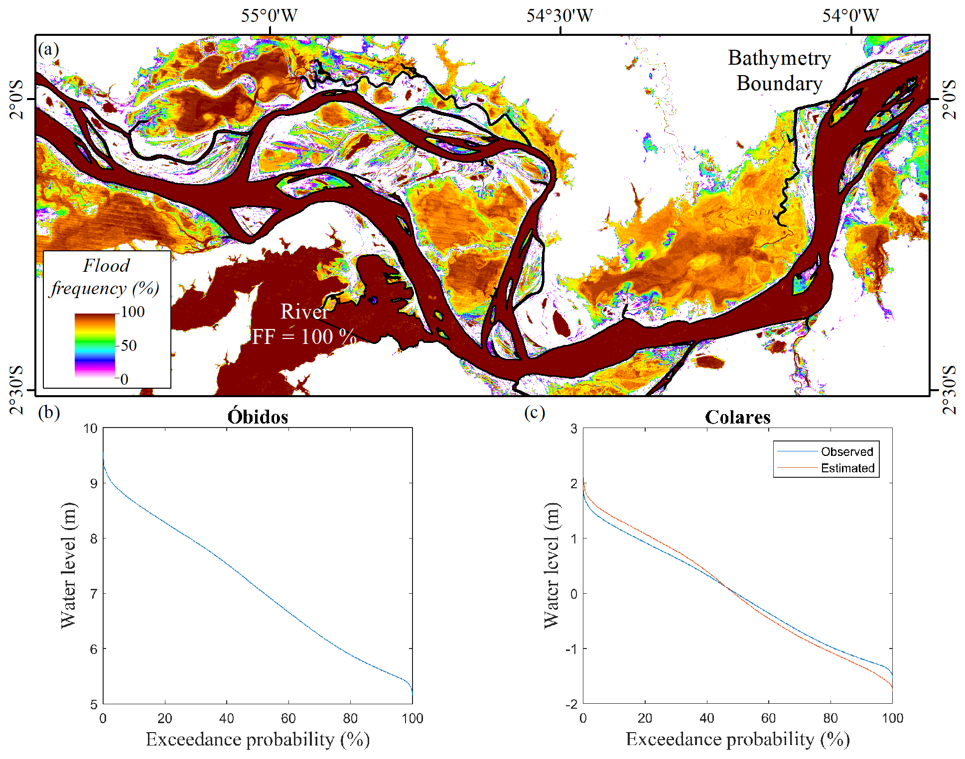
Figure 4(a) Close-up view of the flood frequency map over the Amazon estuary's upstream area. (b) The water level duration function at Óbidos station. (c) The observed and estimated water level duration function at Colares station. (See Fig. 1 for the location of these two stations.)
2.2.1 Riverbanks, intertidal zone, and floodplains
In the intertidal zone and floodplains along the Amazon River, WSE records from limnigraphic and tidal stations were considered over the period from 2015 to 2018 (Tables A2 and A3) for consistency with the imagery period covered by the flood frequency map. These records yielded exceedance probability functions, such as the one illustrated in Fig. 4b (Óbidos station). Like WSE estimation along the river (Sect. 2.1), the water level duration curve was inferred separately along the North Channel and the South Channel (blue lines in Fig. 1) by linearly interpolating the curves obtained at each station. The water level duration curves were then extrapolated via a nearest-neighbor interpolation over the estuary's intertidal areas and floodplains, i.e., everywhere upstream estuary mouths. Therefore, the terrain elevation for any pixel was estimated considering the water level, for which the probability of exceedance is equal to the flood frequency for the same pixel (Fassoni-Andrade et al., 2020b). In permanently flooded areas, i.e., where the flood frequency is 100 %, the method considers the topography equal to the lowest WSE observed, as in the river.
2.2.2 Coastal ocean
The challenge with respect to estimating the topography in the coastal area using the methodology of Fassoni-Andrade et al. (2020b), where vertically leveled tide gauges are lacking, is the inference of spatially distributed water level exceedance functions. We considered the downstream-most Amazon estuary station of Ponta do Céu (Table A2; location in Fig. 1) and computed the water level exceedance function there. This curve's shape was then assumed to be the same throughout the coastal region, although with variable amplitude, proportional to the local tidal amplitude. In this semidiurnal macrotidal region, a reasonable proxy of the tidal amplitude over the region can be thought of as the sum of the amplitudes of the S2 and M2 tidal constituents, as these two constituents are the dominant ones downstream of the river mouth (Gallo and Vinzon, 2005). The water level duration function (WLDF) at any point along the oceanic coastline was obtained by scaling the corresponding function observed at Ponta do Céu (WLDFPC) considering the tidal amplitude given by the S2 and M2 components from the FES2014 model (Carrère et al., 2016), according to Eq. (2):
where the tidal amplitude at a point is given by , and the PC subscript refers to Ponta do Céu values.
As verification, Fig. 4c shows the observed and estimated exceedance probability functions at Colares station, located about 150 km to the east of the Amazon estuary (Fig. 1). Both curves represent the anomaly with respect to the average. The two curves look very similar, with a root-mean-square deviation (RMSD) of 12.7 cm.
After estimating the water level exceedance probability at each point, the vertical reference was adjusted by matching the mean level with the height of the mean sea surface estimated by the ocean circulation model of Ruault et al. (2020). Similar to the water level exceedance probability functions estimated along the river, the coastal area's water level duration functions were inferred for all pixels of the flood frequency map considering the nearest-neighbor interpolation method. Therefore, the terrain elevation for a pixel was estimated considering the water level, for which the probability of exceedance is equal to the flood frequency for the same pixel (Fassoni-Andrade et al., 2020b).
2.3 In situ and spaceborne data for validation
2.3.1 Governo do Estado do Amapá and Exército Brasileiro (GEA/EB) digital terrain model
A digital terrain model (DTM) with a 2.5 m spatial resolution and an accuracy of 1.62 m (BRADAR, 2017), provided by the Instituto de Pesquisas Científicas e Tecnológicas do Estado do Amapá (IEPA; http://www.iepa.ap.gov.br/, last access: 27 January 2021), was used to validate the estimated topography on a sandbank covering ∼ 0.9 km2 in the North Channel (location in Fig. 1). This area was chosen because it is an almost non-vegetated area and it has sufficient corresponding topographic mapping points. For consistency, the DTM vertical reference was transformed from MAPGEO2010 (Matos et al., 2012) to EGM08. The DTM was developed using P-band interferometry from an aerial survey conducted in late 2014 and early 2015 (De Castro-Filho and Antonio Da Silva Rosa, 2017) in the context of the Base Cartográfica Continua do Amapá project (Vieira, 2015) in cooperation with Governo do Estado do Amapá and Exército Brasileiro (GEA/EB).
2.3.2 Ice, Cloud, and land Elevation Satellite-2 (ICESat-2) spaceborne data
The topography was further validated against Ice, Cloud, and land Elevation Satellite-2 (ICESat-2) data. Launched in September 2018, the satellite provides measurements of the surface level from the transmission of laser pulses in the green wavelength (532 nm) by the Advanced Topographic Laser Altimeter System (ATLAS) instrument. ATLAS beams provide six tracks, divided into three pairs, on the Earth surface along the ICESat-2 orbit. The beam pairs are separated by ∼ 3.3 km in the across-track direction, and each spot on the surface has a ∼ 13 m footprint diameter (Neuenschwander et al., 2020). The accuracy expected from ATLAS is approximately 25 cm for flat surfaces and 119 cm in the case of a 10∘ surface slope (Neuenschwander et al., 2020).
The ATL08 version 3 dataset, derived from ATLAS measurements, provides along-track heights above the WGS84 ellipsoid for the land and vegetation every 100 m (available at https://nsidc.org/data/ATL08, last access: 3 August 2020). ATL08 data can also represent water surface elevation; therefore, a criterion has been used to separate these from the measurements over the land surface. Some studies have also shown that the ATLAS instrument can penetrate water and provide information on the bottom (Ma et al., 2020; Parrish et al., 2019). As the Amazon River has a high concentration of sediments (Martinez et al., 2009), we assume that target information from the water only represents the water surface elevation.
Two regions were selected for the validation of topography: upstream of the Xingu River, where the tidal amplitude is small (∼ 40 cm; Kosuth et al., 2009), and along the oceanic coastal area (see Fig. 1 inset map for the locations of both of these regions: “Tidal riverine area” and “Coastal area”, respectively). In both regions, cloudy conditions and measurements with uncertainty above 50 cm (as indicated by the dataset flags) were discarded. Criteria to remove the points derived from the water elevation were considered in each case. In the tidal riverine region, only ATL08 points, converted to EGM08 heights, from the October–December seasons of 2018 and 2019 were considered, as this period represents the low-water season of the Amazon River. Moreover, as the flooded areas should show very low variability in the spaceborne measurements along the track, it is easy to detect them in the individual along-track data. Thus, each track's water level was evaluated, and points below 50 cm above the water elevation were discarded. For the coastal area, tracks with a visually markedly different elevation between ocean and continent were selected. Each selected track was evaluated, and points below 1 m above the water elevation were discarded.
2.3.3 In situ surveys of the riverbed bathymetry
The riverbed was evaluated in six different bathymetry cross sections acquired from past in situ surveys carried out over the 2007–2019 period by SO HYBAM (see https://hybam.obs-mip.fr/, last access: 27 January 2021) and Companhia de Pesquisa de Recursos Minerais (CPRM; location of cross sections in Fig. 1). The water depth was obtained by an acoustic Doppler current profiler (ADCP) instrument, and a WSE was considered here for estimating the bed elevation concerning EGM08. In Section A, we considered the WSE at Óbidos station on the survey day (28 November 2019). In sections, B, C, and D, the WSE at Porto de Moz station on the day of the survey was used and was corrected for each section taking the water surface declivity obtained by the WSE estimated along the river (Fig. 2c) and the distance between the station and section, i.e., WSE at section = WSE at Porto de Moz + WSE slope × distance, into consideration. Finally, the WSE measured every 15 min at Porto de Santana station on 5 June 2008 was considered in sections E and F. As the water level varied by ∼ 50 cm during the time span of these sections, described in Callède et al. (2010), the high-frequency WSE at each point of the sections was considered. Furthermore, metrics were evaluated considering all points (excluding outliers) in the round-trip survey and repetitions. In Section A, four cross sections were acquired; in sections B, C, and D, only one cross section was obtained; and in sections E and F, six and nine cross sections were obtained, respectively.
2.4 Ancillary databases
The estimated topography does not cover the terrain elevation in the non-open-water area. Similarly, our set of bathymetric charts does not cover the Atlantic Ocean's continental shelf downstream of the river mouth. Thus, our dataset was complemented by two global databases: the Multi-Error-Removed Improved-Terrain (MERIT) DEM over the continental area and General Bathymetric Chart of the Oceans (GEBCO) version 2020 over the ocean. MERIT DEM is a widely used global model with a spatial resolution of 90 m in which several errors of the Shuttle Radar Topography Mission (SRTM) DEM and the height of vegetation have been corrected (available at http://hydro.iis.u-tokyo.ac.jp/~yamadai/MERIT_DEM/; Yamazaki et al., 2019). For consistency, the MERIT DEM reference was changed from EGM96 to EGM08 (Pavlis et al., 2012). GEBCO is a global terrain model referred to mean sea level with a spatial resolution of 15 arcsec (approximately 460 m in the Amazon estuary; available at https://www.gebco.net/data_and_products/gridded_bathymetry_data/gebco_2020/, last access: 1 November 2020). As GEBCO data have integer values at intervals of 1 m, the topo-to-raster interpolation was used considering the 1 m isolines to generate data consistent with float values wiping out staircases artifacts. Moreover, a low-pass filter with a 9 point × 9 point and 19 point × 19 point window moving average (i.e., 4.5 km × 4.5 km and 9.5 km × 9.5 km, respectively) was used in the respective regions above (shoreward) and below (off- shoreward) the −200 m isobath to reduce the noise caused by in situ multibeam sounding swaths edges.
These combined databases allowed a unified mapping of the topography and bathymetry of the Amazon estuary. However, as MERIT DEM represents the topography of 2010 and some areas in the coastal region may have been eroded or accreted between 2010 and the 2015–2017 period considered in the flood frequency mapping, a procedure was implemented to correct this issue considering three types of regions: (1) erosion areas; (2) accretion areas, i.e., regions where MERIT product does not have topographic information; and (3) GEBCO regions that represent the continent due to sparse spatial resolution, whereas it should represent transition areas or the ocean. The procedure was performed as follows: (1) MERIT DEM areas with topographic information in eroded areas were selected and replaced by GEBCO data, which cover both the continent and the ocean. In the case of substitution to continent GEBCO data, the region was corrected again in step three. (2) Deposition areas where MERIT does not have topographic information were estimated from the topo-to-raster interpolation method considering the values in the mapped regions' contours. Similarly, (3) GEBCO's high topographic regions in the ocean, including regions not previously corrected in step one, were removed, and new values were estimated by topo-to-raster interpolation considering the neighboring pixels. These areas were manually selected considering the polygons generated from the elevation reclassification into three classes (visually defined criteria): less than −8 m, between −8 and 1 m, and greater than 1 m. Figure A1 shows an example of these steps and a corrected area. Finally, to ensure a smooth transition between the nautical charts and GEBCO, an area was selected and replaced considering topo-to-raster interpolation from the neighboring pixels. This area was defined by a buffer of ∼ 2 km around the transition limit, i.e., considering 4 km width.
3.1 Topography
Figure 5 shows the validation of the estimated topography considering the GEA/EB DTM (“Sandbank” label in Fig. 1) and the ICESat-2 data. The estimated elevation yields an root-mean-square error (RMSE) of 1.15 m, a bias of −0.78 m (standard deviation, SD, of 0.85 m), and a Pearson correlation coefficient (r) of 0.52 (the number of data, n, was 612) compared with GEA/EB DTM. This error may be partly related to the spatial resolution of the Landsat images (30 m) and geomorphological changes in the island during 2014 and 2015, as shown in Fig. 5a and b. Still, this error is lower than the DTM intrinsic accuracy (RMSE of 1.62 m).
Considering the ICESat-2 data, the terrain elevation was also well represented in the riverbanks/floodplain and coastal area, with an r value of 0.8 and 0.8, a RMSE of 1.5 m and 1.8, and a bias of 0.9 m and −1.5, respectively. However, Fig. 5f shows a bias related to the flood frequency in which overestimations are observed at low flood frequencies (e.g., ∼ 3 m for flood frequency of 0 %). As shown in Fassoni-Andrade et al. (2020a), this bias may be related to the Landsat images used in the flood frequency map that do not represent the flood extent in flood-prone vegetated areas. Thus, the flood frequency in these areas is considered only from situations when the water level exceeds the vegetation height; hence, the flood frequency is underestimated, mechanically overestimating the terrain elevation.
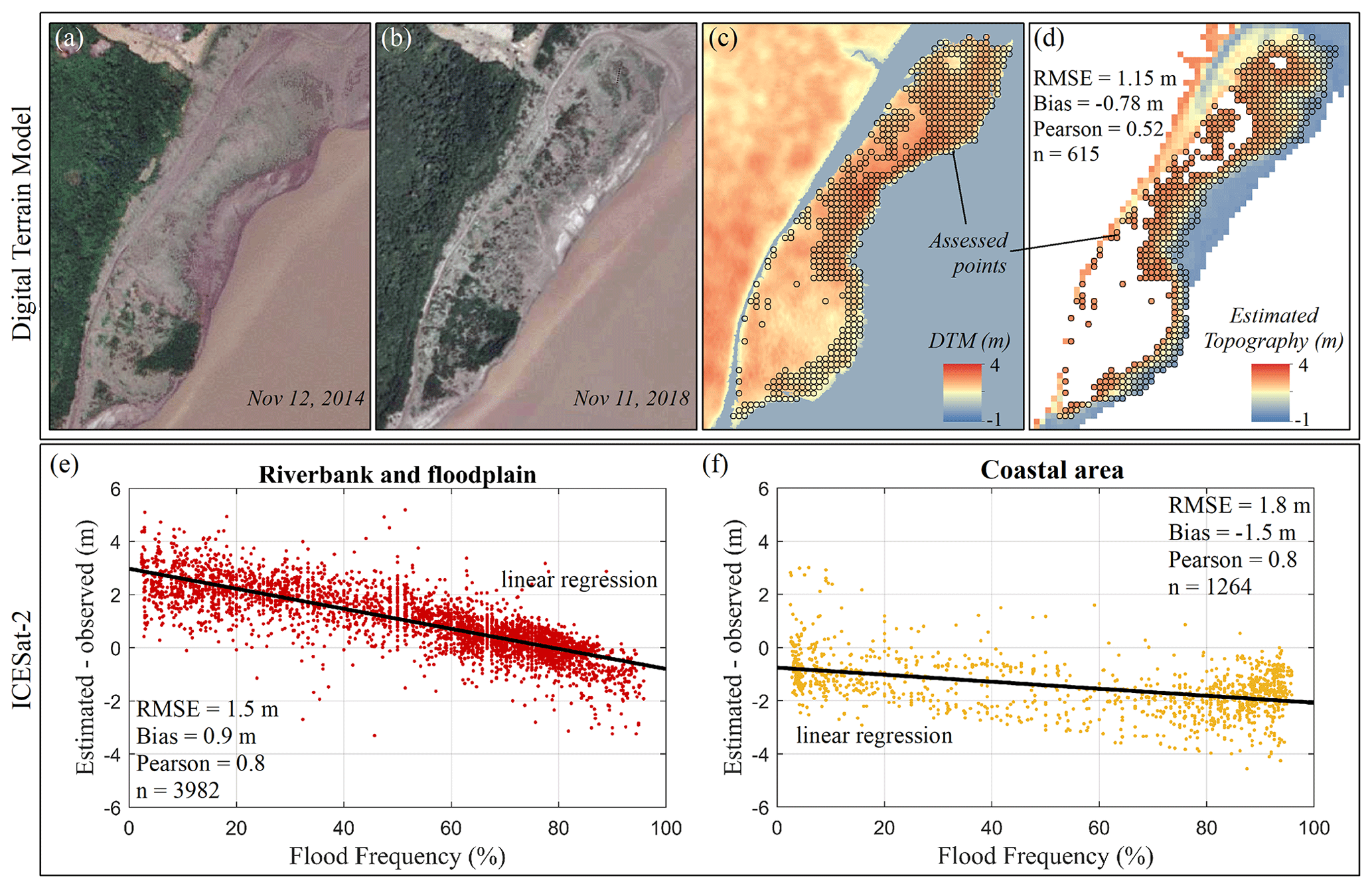
Figure 5Sandbank represented by GEA/EB DTM and topographic mapping (location in Fig. 1). Panels (a) and (b) represent true-color images of the area from Landsat. Panel (c) shows GEA/EB DTM, and panel (d) shows the estimated topography. Flood frequency versus error in topographic estimation in (e) the riverbank/floodplain (“Tidal riverine area” in Fig. 1) and (f) the coastal area (“Coastal area” in Fig. 1) considering the ICESat-2 data.
3.2 Bathymetry
Figure 6 shows the comparison between the in situ cross sections of the Amazon River and our product. The Amazon River's bed elevation was well represented, with an average vertical RMSE of 7.2 m and an average bias of 3.6 m (SD of 5.38 m) for the six sections considered together. Keeping aside the small-scale (typically sub-kilometric) features not resolved by the coarser bathymetric digitized charts, the shape of the cross sections appear appropriately captured by our product, along the steep banks as well as in the median part. The smallest errors are observed in Óbidos (Section A; RMSE of 3.5 m) and North Channel 2 (Section E; RMSE of 2.6 m), possibly due to the shorter time lag between the dates of the surveys (< 5 years) and variation in the bed bathymetry (Vital et al., 1998). Section E, near Macapá city, is over a broad area of overconsolidated sediments, which are difficult to dredge (Vital et al., 1998). Furthermore, the WSEs considered in these sections are from nearby stations, reducing the vertical reference uncertainties.
On the other hand, although the in situ survey for South Channel 2 is about 40 years old (1972–1982; Section F), good agreement appears with the SO HYBAM survey in 2008 (RMSE of 5 m), which shows that the bed surface has possibly not changed much in these 26–36 years.
The region near the Almeirim station, i.e., sections B, C, and D, seems to have undergone the most significant bed change. In general, the errors are larger (e.g., RMSE of 16 m in Section C), and the topographic variation was not represented in the nautical charts. The respective impact of the limited spatial resolution of the digitized nautical charts and of the morphological variability in the bed on the mismatch that we observe is not able to be clearly established in the absence of additional information. These are areas of intense sediment transport with erosion and/or deposition of sand and high variability in the riverbed morphology (Vital et al., 1998). Marked seasonal changes in the riverbed were reported due to extreme net erosion, such as the modification of a channel from a wavy bedform during rising discharge (January 1994) to a flat floor during low discharge (November 1994) with a reduction of up to 7 m in the channel depth (Vital et al., 1998). Therefore, accurate riverbed mapping of this region remains challenging.
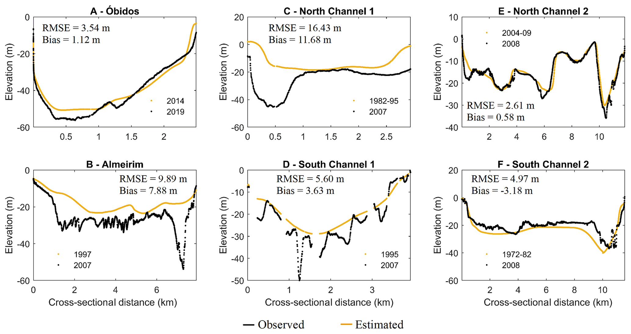
Figure 6Cross-sectional transects of the Amazon River (locations are shown in Fig. 1) from the cross section estimated (yellow) and observed from the in situ surveys (black). Elevations are relative to EGM08. The dates of the corresponding in situ surveys are indicated in each panel.
Figure 7 shows the resulting topography and bathymetry, as well as the complementary MERIT DEM and GEBCO data. The extensive floodplain, riverbanks, and intertidal zone have been seamlessly mapped, as exemplified in boxes A, B, and C. It can be noted that the floodplain extent decreases from the upstream area to the downstream area, and the channels become dendritic in the eastern half of the estuary (east of 52∘ W). This is related to the accumulation of sediment and the fluvial and tidal influences, as described in Fricke et al. (2019) and Nittrouer et al. (2021). These authors showed that the upper estuary, characterized by low tidal influence (∼ 40 cm or less), has high levees that limit the overbank flow and sediment accumulation on the floodplain. In the central reach, the stronger tidal range (∼ 1–2 m) and the associated tidal flow suppress the levees' heights, inducing strong overbank transport with high sedimentation rates on the floodplain. In the lower reach with an even stronger tidal range (∼ 4 m), river-canalized transport predominates, and there is little space for sediment accumulation on the floodplain.
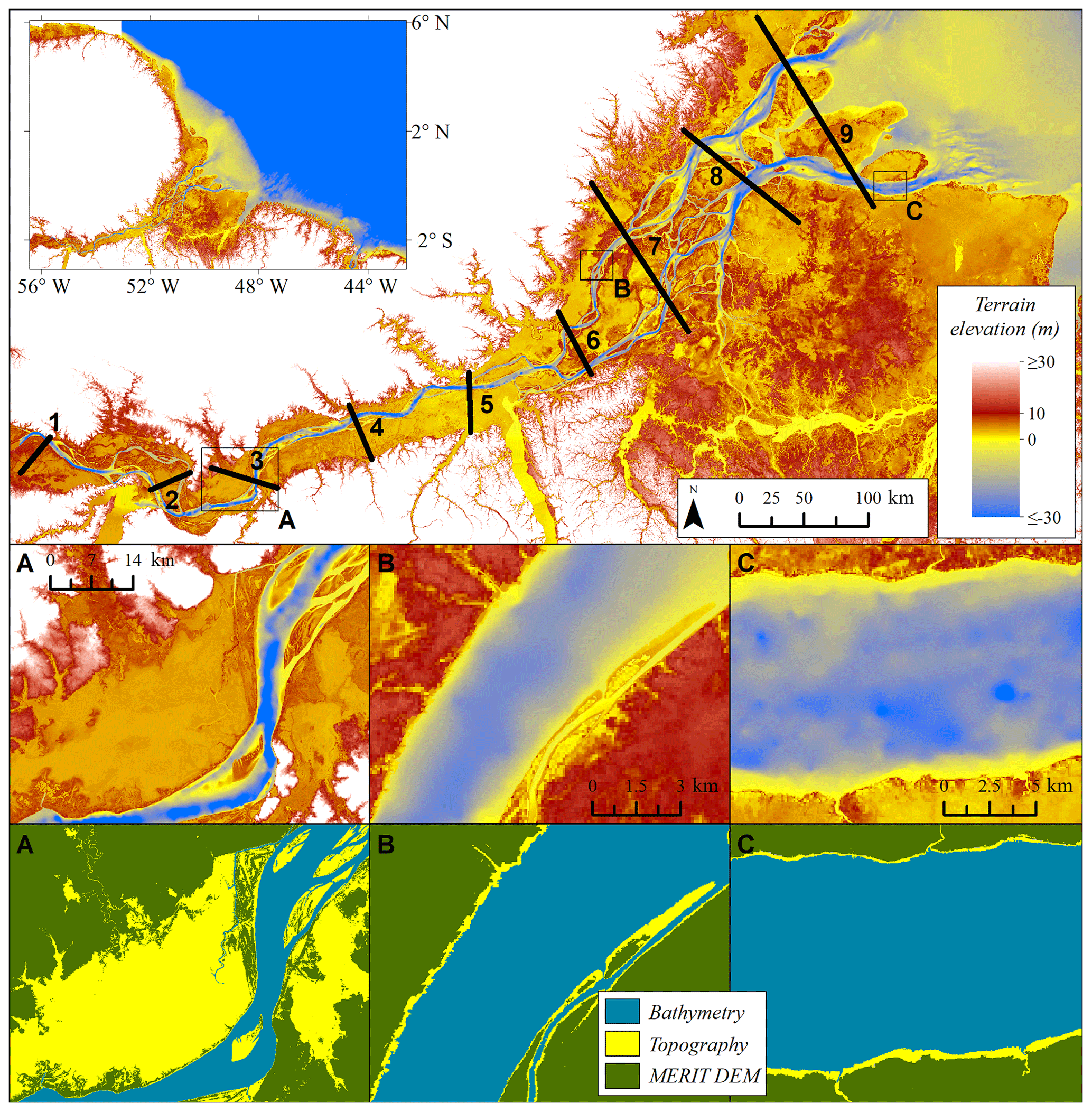
Figure 7Unified topographic mapping of the Amazon estuary (referenced to EGM08): the bathymetry, topography, MERIT, and GEBCO products were merged. The middle row displays close-up views of selected regions. The bottom row indicates the sources of the raw data for the various subdomains.
In general, our product stands under this known geomorphological characterization, which is shown in the nine representative topographic profiles in Fig. 8 (extracted in the across-river direction every 100 km). The color bar represents the flood frequency from the GSW data, i.e., regions where topography and bathymetry were estimated. Black dots represent the MERIT DEM, and the horizontal lines represent the average (blue) and the maximum (red) river WSE (2015–2018). Note that the difference between the average WSE and the floodplain elevation tends to decrease from Section 1 to Section 5 (h values in gray); that is, the space for sediment accommodation on the floodplain decreases due to sediment accumulation. It can also be observed that the height of the levees is similar to the maximum WSE in sections 1 to 5 (upper and central reach), but from Section 6 and further downstream, the topography, represented by the black points, is higher than the maximum elevation and the river has no flooded banks. This observation in the estuary's lower reach has more uncertainty because it considers the MERIT DEM data (Yamazaki et al., 2019), which were not validated here. Fricke et al. (2019) did not observe levees in this reach and described the topography as a flat surface, but the evaluation of the authors considered topographic surveys of the banks with a distance from the river of 30–250 m (average of 80 m), which is equivalent to approximately three points of our analysis (30 m of spatial resolution).
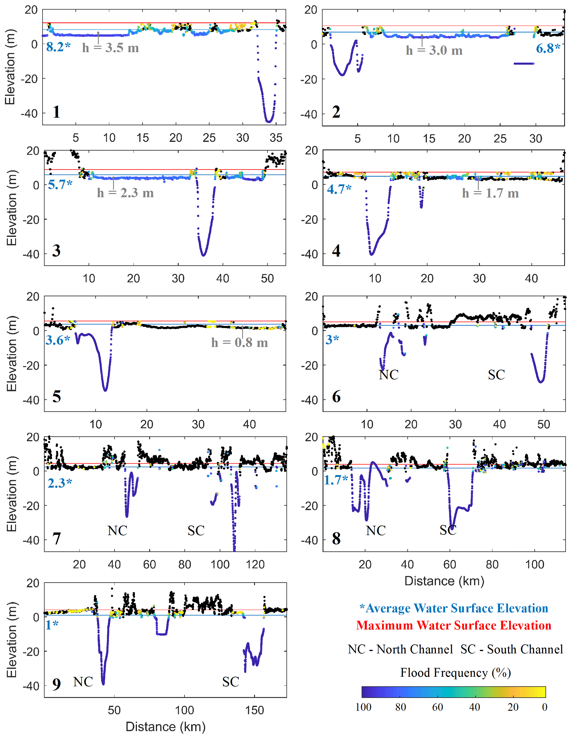
Figure 8Topographic profiles distributed every 100 km along the river, with the flood frequency, average and maximum WSE, and height between the average level and the minimum elevation of the floodplain.
The dataset generated from this work is available at https://doi.org/10.17632/3g6b5ynrdb.2 (Fassoni-Andrade et al., 2021):
-
bathymetry of the Amazon estuary (Bathymetry.tif and Bathymetry.nc) – elevation in meters relative to the EGM2008 geoid;
-
topography of the non-forested portion of the lower Amazon floodplain (Topography.tif and Topography.nc) – elevation in meters relative to the EGM2008 geoid;
-
flood frequency for the period from 2015 to 2018 (FloodFrequency_15to18.tif and FloodFrequency_15to18.nc) – values ranging from 0 % to 100 %;
-
unified mapping of the Amazon estuary – the bathymetry, topography, MERIT, and GEBCO products are merged (DEM_AMestuary.tif and DEM_AMestuary.nc) – elevation in meters relative to the EGM2008 geoid;
-
boundaries of each domain of the unified mapping (domain_boundary.shp);
-
code example to read netcdf files in MATLAB (read_netcdf.m).
All other datasets used in this paper are open-source data cited within.
6.1 Summary and significance of the dataset
Our dataset provides the first ever consistent, high-resolution, vertically referenced topography of the Amazon estuary. Our product's vertical accuracy typically amounts to 7.2 m (bias of 3.6 m) over the riverbed and 1.2 m over non-vegetated intertidal floodplains (2015–2018 period). These values appear to be in line with similar remote, poorly surveyed tropical or deltaic shorelines (Khan et al., 2019; Salameh et al., 2019). Our mapping is based on an innovative approach using remote sensing data, an extensive and novel dataset of river depth, and auxiliary data over the adjoining areas. We believe that this new approach provides unprecedented opportunities for a straightforward estimation of coastal topography worldwide. The validation approach uses an independent and spatially distributed dataset of various origins (in situ and remotely sensed), which provides vital support regarding our findings' quality.
Our overarching goal in assembling this dataset is to characterize the topography and bathymetry of the world's largest estuary. This dataset has many potential applications, such as hydrodynamic modeling, flooding hazard assessment, sedimentology, ecology, and physical or human geography, among others. For hydrodynamic modeling, for instance, where the knowledge of topography is instrumental for the accuracy of the results, as well as for geomorphological assessments, which are usually performed with satellite images extracting horizontal information (e.g., width, length) but most often lacking the vertical information, we believe that this dataset offers a substantial potential for scientific progress. The dataset can also support ecological studies such as vegetation distribution and carbon balance.
The availability of high-resolution spaceborne imagery promised by ongoing operational initiatives, such as the European Sentinel program or the upcoming Constellation Optique 3D (CO3D) mission, provides excellent prospects for frequent revisit updates and improvement of the intertidal part of our product. Keeping the Amazon estuary's energetic morphodynamics in mind , such updates will ensure a perennial quality of our dataset.
6.2 Caveats
Our product's main limitation lies in the long time span of our raw bathymetry data collection (encompassing 5 decades, Table A1). This limitation is probably sensible regarding the supposed characteristic timescale of the variability in the riverbed through erosion and accretion processes, as revealed from our validation. Repeated shipborne bathymetric surveys are needed, although the geographical extent of the domain makes it hardly tractable at this mega-delta scale. In particular, it would be opportune to consider the future releases of bathymetric charts by the Brazilian Navy along the Amazon estuary, as they become available in the future years, in case they are based on updated primary bathymetric surveys. The issue is less severe for the intertidal topography, as the time span of our primary data period is inferior by 1 order of magnitude (4 years only). Inherently, our product relies on the GEBCO digital terrain model in the open-ocean region. As such, we are subject to the same sources of error as everywhere else in the world ocean, related to the poor knowledge of the vertical datum of some of the primary data used in the GEBCO composite product (Weatherall et al., 2015). Our product is also potentially impacted by the inhomogeneity of the quality of the GEBCO digital terrain model, in particular in the near-shore oceanic regions (Amante and Eakins, 2016).
Another limitation of our dataset over the intertidal flats and floodplains results from the approach based on remotely sensed imagery of GSW product to estimate the flood frequency. Indeed, it is not expected to work well over the Amazon estuary areas that are densely vegetated. In addition, topographic mapping bias due to flooded vegetation could be avoided by using satellite radar data to map the water extent even in flooded vegetation, such as ALOS–PALSAR (Advanced Land Observing Satellite–Phased Array type L-band Synthetic Aperture Radar; Arnesen et al., 2013). Another issue with using Landsat images for coastal topography estimation is that the flood extent representation is only every 16 d (Landsat has a sun-synchronous orbit). The tide's temporal variability occurs on an hourly scale, and the amplitude of the S2 tidal constituent would be observed in the same phase, introducing a bias in the mapping. More investigations are needed using images with more significant temporal variability. The upcoming Surface Water and Ocean Topography (SWOT) satellite mission that will provide, for the first time, frequent mapping of the water surface elevation and water extent over continental and riverine areas offers a bright prospect to curb these limitations.
Table A1Identification of nautical charts and dates of surveys (Brazilian Navy).
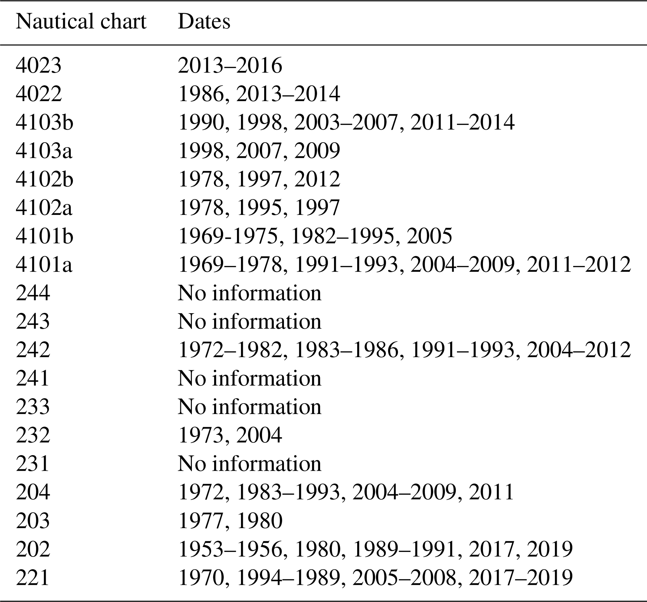
Table A2Gauge station in the North Channel of the Amazon estuary.
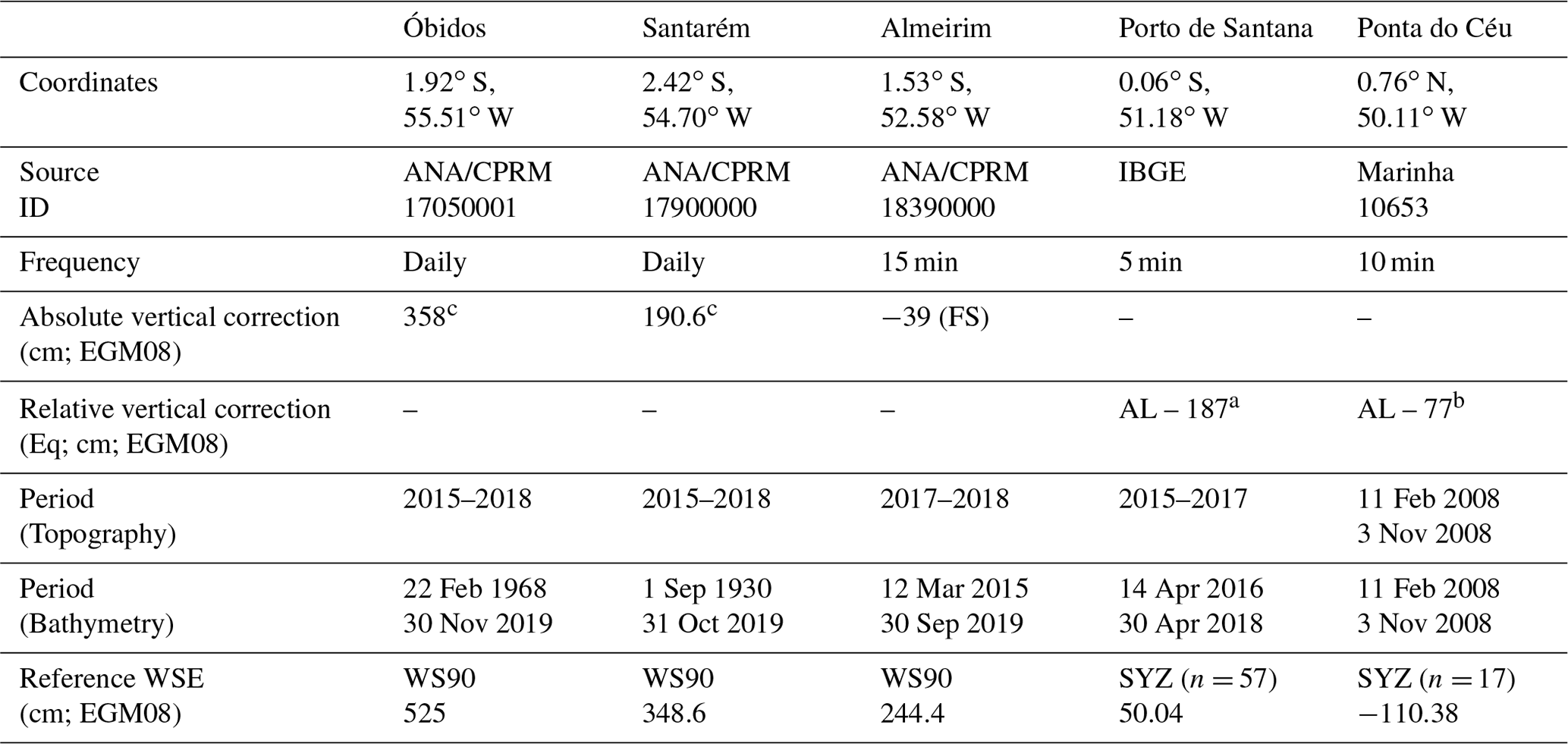
FS stands for field survey (Appendix A), and Eq denotes average level (AL) – level above the geoid (EGM08). a Callède et al. (2013). b Ruault et al. (2020). c Calmant et al. (2013).
Series of stage values are relative to a so-called “gauge zero”, which simply corresponds to the lowest mark on the graduated staff and is referred to an arbitrary datum that is different for each gauge station. Therefore, stages from one gauge cannot be compared in an absolute way to stages from other gauges. It is not possible to obtain the corresponding water surface elevation to derive, for example, the slope of the water surface or relate the water level to a digital elevation model of the surrounding watershed. However, the slope information is a key parameter for the hydrodynamic modeling of the flow in the basin. The “zero values” of the Almeirim and Porto de Moz gauge stations were surveyed using GNSS (Global Navigation Satellite System) geodetic receivers installed over gauges benchmarks. The data surveyed were computed with the precise point positioning (PPP) technique (Héroux and Kouba, 1995), using the GINS software (Marty et al., 2011) developed by the French Space Agency (CNES). Coordinates were produced in the WGS84 ellipsoid related with the ITRF2014 frame and following all of the recommended corrections from the International Earth Rotation and Reference Systems Service (IERS) 2010 conventions (McCarthy and Petit, 2004). The efficiency and accuracy of GINS to process GPS data in the PPP mode expected from our processing chain is better than 2 cm. This expected accuracy is possible thanks to the GNSS observation time and the model corrections' accuracy (see Moreira et al., 2016, for further details).
Table A3Gauge station in the South Channel of the Amazon estuary.
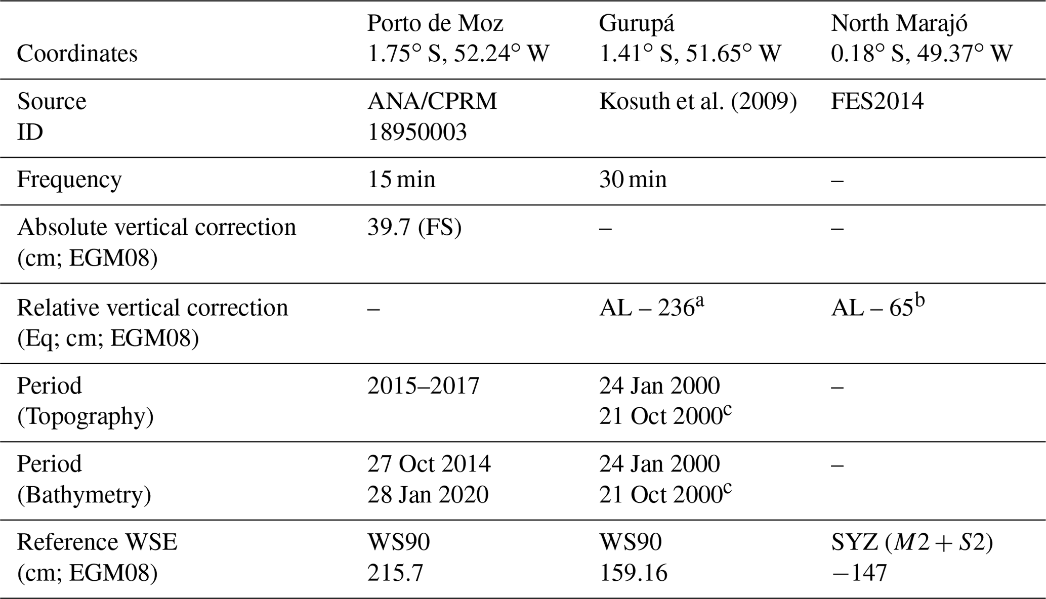
FS stands for field survey (Appendix A), and Eq denotes average level (AL) – level above the geoid (EGM08). a Callède et al. (2013). b Ruault et al. (2020). c Data from October 2000 are repeated twice to complete 1 year of data.
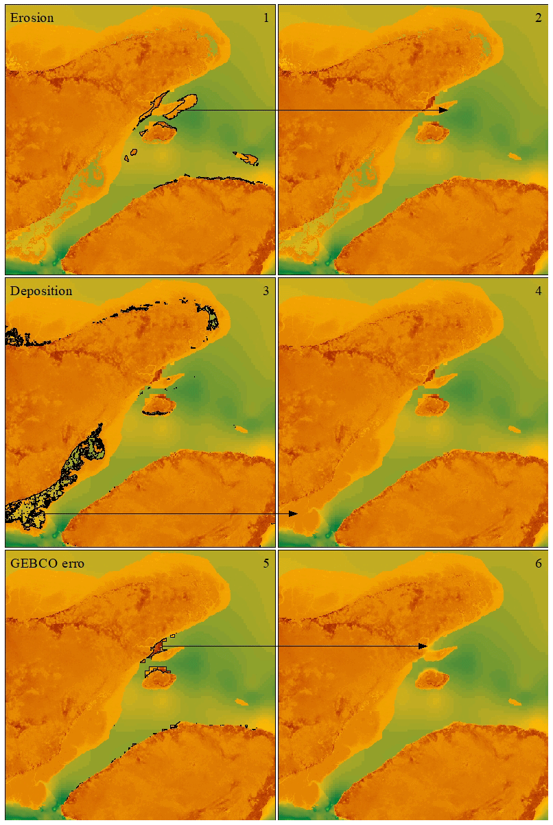
Figure A1An example of data correction in the ocean after merging the database (GEBCO, MERIT DEM, bathymetry, and topography).
AF and FD conceptualized the study, acquired data, undertook the formal analysis, and were responsible for developing the methodology, undertaking data validation, and writing, reviewing, and editing the paper. DM acquired data and was responsible for developing the methodology, undertaking data validation, and writing, reviewing, and editing the paper. AA was responsible for developing the methodology, undertaking data validation, project administration, and writing, reviewing, and editing the paper. VF, CF, and AL acquired data and wrote, reviewed, and edited the paper.
The authors declare that they have no conflict of interest.
The authors acknowledge financial support from EOSC, IRD, CPRM, and LAGEQ/IG/UnB. Leandro Guedes Santos (CPRM-Belém), Rodrigo Da Silva (UFOPA – Santarém), Fabrice Papa (IRD-LEGOS), Victor Hugo da Motta Paca (CPRM-Belém), Arthur Abreu (CPRM-Rio de Janeiro), and the whole crew of the R/V Isabella are thanked for logistical support during the “Dinâmica Fluvial 2020” bathymetric cruise. The authors are grateful to Gérard Cochonneau (from SO HYBAM-IRD) for sharing the in situ tidal records published by Kosuth et al. (2009) and to Julien Jouanno (IRD-LEGOS) for sharing the mean sea surface of the ocean circulation model of Ruault et al. (2020).
This research has been supported by Horizon 2020 (EOSC-synergy, grant no. 857647).
This paper was edited by Giuseppe M. R. Manzella and reviewed by Panagiotis Agrafiotis, Marco Ligi, Thierry Schmitt, and one anonymous referee.
Amante, C. J. and Eakins, B. W.: Accuracy of interpolated bathymetry in digital elevation models, in: Advances in Topobathymetric Mapping, Models, and Applications, vol. 76, edited by: Brock, J. C., Gesch, D. B., Parrish, C. E., Rogers, J. N., and Wright, C. W., Journal of Coastal Research, Coconut Creek (Florida), 123–133, 2016.
Andrade, M. M. N. and Szlafsztein, C. F.: Vulnerability assessment including tangible and intangible components in the index composition: An Amazon case study of flooding and flash flooding, Sci. Total Environ., 630, 903–912, https://doi.org/10.1016/j.scitotenv.2018.02.271, 2018.
Armon, M., Dente, E., Shmilovitz, Y., Mushkin, A., Cohen, T. J., Morin, E., and Enzel, Y.: Determining Bathymetry of Shallow and Ephemeral Desert Lakes Using Satellite Imagery and Altimetry, Geophys. Res. Lett., 47, 1–9, https://doi.org/10.1029/2020GL087367, 2020.
Arnesen, A. S., Silva, T. S. F. F., Hess, L. L., Novo, E. M. L. M. L. M., Rudorff, C. M., Chapman, B. D., and McDonald, K. C.: Monitoring flood extent in the lower Amazon River floodplain using ALOS/PALSAR ScanSAR images, Remote Sens. Environ., 130, 51–61, https://doi.org/10.1016/j.rse.2012.10.035, 2013.
Bell, P. S., Bird, C. O., and Plater, A. J.: A temporal waterline approach to mapping intertidal areas using X-band marine radar, Coast. Eng., 107, 84–101, https://doi.org/10.1016/j.coastaleng.2015.09.009, 2016.
Bergmann, M., Durand, F., Krien, Y., Khan, M. J. U., Ishaque, M., Testut, L., Calmant, S., Maisongrande, P., Islam, A. K. M. S., Papa, F., and Ouillon, S.: Topography of the intertidal zone along the shoreline of Chittagong (Bangladesh) using PROBA-V imagery, Int. J. Remote Sens., 39, 9004–9024, https://doi.org/10.1080/01431161.2018.1504341, 2018.
Bishop-Taylor, R., Sagar, S., Lymburner, L., and Beaman, R. J.: Between the tides: Modelling the elevation of Australia's exposed intertidal zone at continental scale, Estuar. Coast. Shelf Sci., 223, 115–128, https://doi.org/10.1016/j.ecss.2019.03.006, 2019.
BRADAR: Projeto DSG AMAPÁ relatório técnico processamento SAR v.1., 2017.
Callède, J., Cochonneau, G., Alves, F. V., Guyot, J.-L., Guimarães, V. S., and De Oliveira, E.: The River Amazon water contribution to the Atlantic Ocean, Rev. des Sci. l'eau, 23, 247–273, https://doi.org/10.7202/044688ar, 2010.
Callède, J., Moreira, D. M., and Calmant, S.: Détermination de l'altitude du zéro des stations hydrométriques en amazonie brésilienne, Application aux lignes d'eau des Rios Negro, Solimões et Amazone, Rev. des Sci. l'Eau, 26, 153–171, https://doi.org/10.7202/1016065ar, 2013.
Calmant, S., Da Silva, J. S., Moreira, D. M., Seyler, F., Shum, C. K., Crétaux, J. F., and Gabalda, G.: Detection of Envisat RA2/ICE-1 retracked radar altimetry bias over the Amazon basin rivers using GPS, Adv. Sp. Res., 51, 1551–1564, https://doi.org/10.1016/j.asr.2012.07.033, 2013.
Carrère, L., Lyard, F. H., Cancet, M., Guillot, A., and Picot, N.: Finite Element Solution FES2014, a new tidal model – Validation results and perspectives for improvements, in: ESA Living Planet Conference, Prague, 9–13 May 2016.
De Castro-Filho, C. A. P. and Antonio Da Silva Rosa, R.: Brazilian Amazon land mapping project: Status and perspectives, in: International Geoscience and Remote Sensing Symposium (IGARSS), Fort Worth, TX, 23–28 July 2017, 2895–2898, 2017.
Dai, C., Howat, I. M., Larour, E., and Husby, E.: Coastline extraction from repeat high resolution satellite imagery, Remote Sens. Environ., 229, 260–270, https://doi.org/10.1016/j.rse.2019.04.010, 2019.
Dyer, K. R.: Estuaries: a physical introduction, Wiley-Interscience, London, 1997.
Fassoni-Andrade, A. C., Paiva, R. C. D., Rudorff, C. M., Barbosa, C. C. F. and Novo, E. M. L. d. M.: High-resolution mapping of floodplain topography from space: A case study in the Amazon, Remote Sens. Environ., 251, 112065, https://doi.org/10.1016/j.rse.2020.112065, 2020a.
Fassoni-Andrade, A. C., Paiva, R. C. D., and Fleischmann, A. S.: Lake topography and active storage from satellite observations of flood frequency, Water Resour. Res., 56, e2019WR026362, https://doi.org/10.1029/2019wr026362, 2020b.
Fassoni-Andrade, A., Durand, F., Moreira, D., Azevedo, A., Santos, V., Funi, C. and Laraque, A.: Comprehensive bathymetry and intertidal topography of the Amazon estuary, Mendeley Data, V2, https://doi.org/10.17632/3g6b5ynrdb.2, 2021.
Fernandes, R. D., Vinzon, S. B. and De Oliveira, F. A. M.: Navigation at the Amazon River mouth: Sand bank migration and depth surveying, 11th Triennial International Conference on Ports, San Diego, California, USA, 25-28 March 2007, https://doi.org/10.1061/40834(238)52, 2007.
Filizola, N., Guyot, J.-L., Wittmann, H., Martinez, J.-M. and de Oliveira, E.: The Significance of Suspended Sediment Transport Determination on the Amazonian Hydrological Scenario, in: Sediment Transport in Aquatic Environments, edited by: Manning, A. J., IntechOpen, https://doi.org/10.5772/19948, 2011.
Fricke, A. T., Nittrouer, C. A., Ogston, A. S., Nowacki, D. J., Asp, N. E., and Souza Filho, P. W. M.: Morphology and dynamics of the intertidal floodplain along the Amazon tidal river, Earth Surf. Process. Land., 44, 204–218, https://doi.org/10.1002/esp.4545, 2019.
Gabioux, M., Vinzon, S. B., and Paiva, A. M.: Tidal propagation over fluid mud layers on the Amazon shelf, Cont. Shelf Res., 25, 113–125, https://doi.org/10.1016/j.csr.2004.09.001, 2005.
Gallo, M. N. and Vinzon, S. B.: Generation of overtides and compound tides in Amazon estuary, Ocean Dyn., 55, 441–448, https://doi.org/10.1007/s10236-005-0003-8, 2005.
Gallo, M. N. and Vinzon, S. B.: Estudo numérico do escoamento em planícies de marés do canal Norte (estuário do rio Amazonas), Ribagua, 2, 38–50, https://doi.org/10.1016/j.riba.2015.04.002, 2015.
Gorelick, N., Hancher, M., Dixon, M., Ilyushchenko, S., Thau, D., and Moore, R.: Google Earth Engine: Planetary-scale geospatial analysis for everyone, Remote Sens. Environ., 202, 18–27, https://doi.org/10.1016/j.rse.2017.06.031, 2017.
Héroux, P. and Kouba, J.: GPS precise point positioning with a difference, Geomatics'95, Ottawa, Canada, 13–15 June 1995, 1995.
Hutchinson, M. F.: A new procedure for gridding elevation and stream line data with automatic removal of spurious pits, J. Hydrol., 106, 211–232, https://doi.org/10.1016/0022-1694(89)90073-5, 1989.
Khan, J. U., Ansary, N., and Durand, F.: High-Resolution Intertidal Topography from Sentinel-2 Multi-Spectral Imagery: Synergy between Remote Sensing and Numerical Modeling, 11, 2888, https://doi.org/10.3390/rs11242888, 2019.
Kosuth, P., Callede, J., Laraque, A., Filizola, N., Guyot, J. L., Seyler, P., Fritsch, J. M., and Guimarães, V.: Sea-tide effects on flows in the lower reaches of the Amazon River, Hydrol. Process., 23, 3141–3150, https://doi.org/10.1002/hyp.7387, 2009.
Latrubesse, E. M., Arima, E. Y., Dunne, T., Park, E., Baker, V. R., D'Horta, F. M., Wight, C., Wittmann, F., Zuanon, J., Baker, P. A., Ribas, C. C., Norgaard, R. B., Filizola, N., Ansar, A., Flyvbjerg, B., and Stevaux, J. C.: Damming the rivers of the Amazon basin, Nature, 546, 363–369, https://doi.org/10.1038/nature22333, 2017.
Ma, Y., Xu, N., Liu, Z., Yang, B., Yang, F., Wang, X. H., and Li, S.: Satellite-derived bathymetry using the ICESat-2 lidar and Sentinel-2 imagery datasets, Remote Sens. Environ., 250, 112047, https://doi.org/10.1016/j.rse.2020.112047, 2020.
Mansur, A. V., Brondízio, E. S., Roy, S., Hetrick, S., Vogt, N. D., and Newton, A.: An assessment of urban vulnerability in the Amazon Delta and Estuary: a multi-criterion index of flood exposure, socio-economic conditions and infrastructure, Sustain. Sci., 11, 625–643, https://doi.org/10.1007/s11625-016-0355-7, 2016.
Martinez, J. M., Guyot, J. L., Filizola, N., and Sondag, F.: Increase in suspended sediment discharge of the Amazon River assessed by monitoring network and satellite data, Catena, 79, 257–264, https://doi.org/10.1016/j.catena.2009.05.011, 2009.
Marty, J. C., Loyer, S., Perosanz, F., Mercier, F., Bracher, G., Legresy, B., Portier, L., Capdeville, H., Fund, F., Lemoine, J. M., and Biancale, R.: GINS the CNESGRGS GNSS scientific software, in: 3rd International colloquium scientific and fundamental aspects of the Galileo programme, Copenhagen, Denmark, 31 August–2 September 2011, ESA proceedings WPP326, 31, 8–10, 2011.
Matos, A. C. O. C. d., Blitzkow, D., Guimarães, G. d. N., Lobianco, M. C. B., and Costa, S. M. A.: Validação do MAPGEO2010 e comparação com modelos do geopotencial recentes, Bol. Ciências Geodésicas, 18, 101–122, https://doi.org/10.1590/s1982-21702012000100006, 2012.
McCarthy, D. D. and Petit, G.: IERS Technical Note# 32—IERS Conventions (2003), Frankfurt, 2004.
Molinas, E., Vinzon, S. B., de Paula Xavier Vilela, C., and Gallo, M. N.: Structure and position of the bottom salinity front in the Amazon Estuary, Ocean Dyn., 64, 1583–1599, https://doi.org/10.1007/s10236-014-0763-0, 2014.
Molinas, E., Carneiro, J. C., and Vinzon, S.: Internal tides as a major process in Amazon continental shelf fine sediment transport, Mar. Geol., 430, 106360, https://doi.org/10.1016/j.margeo.2020.106360, 2020.
Moreira, D. M., Calmant, S., Perosanz, F., Xavier, L., Rotunno Filho, O. C., Seyler, F., and Monteiro, A. C.: Comparisons of observed and modeled elastic responses to hydrological loading in the Amazon basin, Geophys. Res. Lett., 43, 9604–9610, https://doi.org/10.1002/2016GL070265, 2016.
Neuenschwander, A. L., Pitts, K. L., Jelley, B. P., Robbins, J., Klotz, B., Popescu, S. C., Nelson, R. F., Harding, D., Pederson, D., and Sheridan, R.: ATLAS/ICESat-2 L3A Land and Vegetation Height, Version 3. ATL08, NASA National Snow and Ice, Boulder, CO, USA, 2020.
Nittrouer, C., DeMaster, D., Kuehl, S., Figueiredo, A., Sternberg, R., Faria, L. E. C., Silveira, O., Allison, M., Kineke, G., Ogston, A., Souza Filho, P., Asp, N., Nowacki, D. and Fricke, A.: Amazon Sediment Transport and Accumulation Along the Continuum of Mixed Fluvial and Marine Processes, Ann. Rev. Mar. Sci., 13, 1–36, https://doi.org/10.1146/annurev-marine-010816-060457, 2021.
Parrish, C. E., Magruder, L. A., Neuenschwander, A. L., Forfinski-Sarkozi, N., Alonzo, M., and Jasinski, M.: Validation of ICESat-2 ATLAS bathymetry and analysis of ATLAS's bathymetric mapping performance, Remote Sens., 11, 1634, https://doi.org/10.3390/rs11141634, 2019.
Pavlis, N. K., Holmes, S. A., Kenyon, S. C., and Factor, J. K.: The development and evaluation of the Earth Gravitational Model 2008 (EGM2008), J. Geophys. Res.-Sol. Ea., 117, B04406, https://doi.org/10.1029/2011JB008916, 2012.
Pekel, J.-F., Cottam, A., Gorelick, N., and Belward, A. S.: High-resolution mapping of global surface water and its long-term changes, Nature, 540, 418–422, https://doi.org/10.1038/nature20584, 2016.
Prestes, Y. O., Borba, T. A. da C., Silva, A. C. d., and Rollnic, M.: A discharge stationary model for the Pará-Amazon estuarine system, J. Hydrol. Reg. Stud., 28, 100668, https://doi.org/10.1016/j.ejrh.2020.100668, 2020.
Pugh, D. and Woodworth, P.: Sea-Level Science: Understanding Tides, Surges, Tsunamis and Mean Sea-Level Changes, 2014.
Ruault, V., Jouanno, J., Durand, F., Chanut, J., and Benshila, R.: Role of the Tide on the Structure of the Amazon Plume: A Numerical Modeling Approach, J. Geophys. Res.-Ocean., 125, 1–17, https://doi.org/10.1029/2019jc015495, 2020.
Salameh, E., Frappart, F., Almar, R., Baptista, P., Heygster, G., Lubac, B., Raucoules, D., Almeida, L. P., Bergsma, E. W. J., Capo, S., De Michele, M. D., Idier, D., Li, Z., Marieu, V., Poupardin, A., Silva, P. A., Turki, I., and Laignel, B.: Monitoring Beach Topography and Nearshore Bathymetry Using Spaceborne Remote Sensing: A Review, Remote Sens., 11, 2212, https://doi.org/10.3390/rs11192212, 2019.
Salameh, E., Frappart, F., Turki, I., and Laignel, B.: Intertidal topography mapping using the waterline method from Sentinel-1 & -2 images: The examples of Arcachon and Veys Bays in France, ISPRS J. Photogramm. Remote Sens., 163, 98–120, https://doi.org/10.1016/j.isprsjprs.2020.03.003, 2020.
Sawakuchi, H. O., Neu, V., Ward, N. D., Barros, M. d. L. C., Valerio, A. M., Gagne-Maynard, W., Cunha, A. C., Less, D. F. S., Diniz, J. E. M., Brito, D. C., Krusche, A. V., and Richey, J. E.: Carbon Dioxide Emissions along the Lower Amazon River, Front. Mar. Sci., 4, 76, https://doi.org/10.3389/fmars.2017.00076, 2017.
Tseng, K. H., Kuo, C. Y., Lin, T. H., Huang, Z. C., Lin, Y. C., Liao, W. H., and Chen, C. F.: Reconstruction of time-varying tidal flat topography using optical remote sensing imageries, ISPRS J. Photogramm. Remote Sens., 131, 92–103, https://doi.org/10.1016/j.isprsjprs.2017.07.008, 2017.
Vieira, M. S.: Base cartográfica contínua do estado do Amapá, Rev. Digit. Simonsen, 3, 47–60, 2015.
Vital, H., Stattegger, K., Posewang, J., and Theilen, F.: Lowermost Amazon River: Morphology and shallow seismic characteristics, Mar. Geol., 152, 277–294, https://doi.org/10.1016/S0025-3227(98)00099-1, 1998.
Ward, N. D., Krusche, A. V., Sawakuchi, H. O., Brito, D. C., Cunha, A. C., Moura, J. M. S., da Silva, R., Yager, P. L., Keil, R. G., and Richey, J. E.: The compositional evolution of dissolved and particulate organic matter along the lower Amazon River-Óbidos to the ocean, Mar. Chem., 177, 244–256, https://doi.org/10.1016/j.marchem.2015.06.013, 2015.
Weatherall, P., Marks, K. M., Jakobsson, M., Schmitt, T., Tani, S., Arndt, J. E., Rovere, M., Chayes, D., Ferrini, V., and Wigley, R.: A new digital bathymetric model of the world's oceans, Earth Sp. Sci., 2, 331–345, https://doi.org/10.1002/2015EA000107, 2015.
Yamazaki, D., Ikeshima, D., Sosa, J., Bates, P. D., Allen, G. H., and Pavelsky, T. M.: MERIT Hydro: A High-Resolution Global Hydrography Map Based on Latest Topography Dataset, Water Resour. Res., 55, 5053–5073, https://doi.org/10.1029/2019WR024873, 2019.