The Global Streamflow Indices and Metadata Archive (GSIM) – Part 2: Quality control, time-series indices and homogeneity assessment

This is Part 2 of a two-paper series presenting the Global Streamflow Indices and Metadata Archive (GSIM), which is a collection of daily streamflow observations at more than 30 000 stations around the world. While Part 1 (Do et al., 2018a) describes the data collection process as well as the generation of auxiliary catchment data (e.g. catchment boundary, land cover, mean climate), Part 2 introduces a set of quality controlled time-series indices representing (i) the water balance, (ii) the seasonal cycle, (iii) low flows and (iv) floods. To this end we first consider the quality of individual daily records using a combination of quality flags from data providers and automated screening methods. Subsequently, streamflow time-series indices are computed for yearly, seasonal and monthly resolution. The paper provides a generalized assessment of the homogeneity of all generated streamflow time-series indices, which can be used to select time series that are suitable for a specific task. The newly generated global set of streamflow time-series indices is made freely available with an digital object identifier at https://doi.pangaea.de/10.1594/PANGAEA.887470 and is expected to foster global freshwater research, by acting as a ground truth for model validation or as a basis for assessing the role of human impacts on the terrestrial water cycle. It is hoped that a renewed interest in streamflow data at the global scale will foster efforts in the systematic assessment of data quality and provide momentum to overcome administrative barriers that lead to inconsistencies in global collections of relevant hydrological observations.

1 Introduction

Although terrestrial freshwater is an essential component of the Earth system and a prerequisite for societal development, the availability of relevant in situ observations at the global scale has been limited. Until now, most relevant in situ observations have been held by national and regional authorities, and despite their best efforts, international data centres only have access to a small subset of the full observed record (Do et al., 2018a). This situation stands in contrast to the fact that monitoring data are increasingly being made publicly available through regional and national authorities (Do et al., 2018a). In this paper series, we present an international collection of river and streamflow observations that covers more than 30 000 stations around the globe, highlighting the fact that these are among the best monitored variables of the terrestrial water cycle (Fekete et al., 2012, 2015; Gudmundsson and Seneviratne, 2015; Hannah et al., 2011). Part 1 of the paper series (Do et al., 2018a) documents the data-collection process together with a meta-database that allows users to recreate the collection from the original data sources. In addition, Part 1 of this paper series also presents auxiliary data including catchment boundaries delineated from global digital elevation models as well as selected properties (e.g. land cover, climate) of these catchments.

While the data collection outlined in Part 1 (Do et al., 2018a) increases the spatial and temporal availability of streamflow records at the global scale, it is important to also consider the quality of the data. This is especially relevant for this merged data product combining information from several databases, which might have been set up with different objectives. Furthermore, data contained in individual databases may stem from different sources, often with unknown quality control procedures. In addition, changes in instrumentation as well as human impacts such as stream straightening or flow regulations can have pronounced effects on the observed record. Establishing a database of quality controlled streamflow observations is therefore essential for many applications, including e.g. the need to evaluate the increasing number of continental- and global-scale hydrological and land-surface models that have emerged in recent decades (Beck et al., 2017; Gudmundsson et al., 2012a, b; Haddeland et al., 2011; Zaitchik et al., 2010) and the assessment of human impacts on the terrestrial water cycle (Alkama et al., 2013; Barnett et al., 2008; Destouni et al., 2013; Gudmundsson et al., 2017; Hegerl et al., 2015; Hidalgo et al., 2009; Jaramillo and Destouni, 2015; Oliveira et al., 2011). While there have been significant efforts in the climatological community to share and standardize transnational weather observations as well as derivative data products (Alexander et al., 2006; Becker et al., 2013; Dee et al., 2011; Harris et al., 2014; Haylock et al., 2008; Poli et al., 2016), the hydrological community has traditionally been reticent to adopt regional or global approaches, instead focussing predominantly on the catchment scale. A more concerted and coordinated effort to understand the quality of streamflow observations across the globe provides significant opportunities for fostering hydrological research in support of understanding of global water budgets. This paper initiates the process of evaluating, analysing and documenting the quality of observed streamflow time series, providing a method for increasing the reliability and ongoing value of the database. To do so, this paper expands on previous research (Gudmundsson and Seneviratne, 2016) and applies a set of transparent and reproducible methods to evaluate the quality of the considered records.

One limitation of the newly assembled collection of daily river flow and streamflow time series is that publication of unprocessed daily values is restricted for some of the original data sources. To nevertheless be able to publish relevant information on observational streamflow, we therefore present here processed data in the form of time-series indices that capture essential aspects of (i) the water balance, (ii) seasonality, (iii) low flows and (iv) floods. The approach of publishing time-series indices instead of raw daily values is adapted from the CCl/WCRP/JCOMM Expert Team on Climate Change Detection and Indices (ETCCDI) (https://www.wcrp-climate.org/data-etccdi), which has developed this approach to make relevant climate information publicly available in cases where access to raw daily values is restricted. The ETCCDI has focussed on indices characterizing changes in extreme precipitation and temperature, based on a core collection of indices proposed by Frich et al. (2002). Both Klein Tank et al. (2009) and Zhang et al. (2011) provide additional background on the usage and computation of the ETCCDI indices. Klein Tank et al. (2009) also provide guidelines for quality control of the raw daily input data, index computation and assessment of time-series homogeneity.

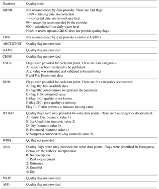
Table 1 Quality flags of daily values of all databases that enter the GSIM collection (see Do et al., 2018a).

The use of time-series indices for characterizing the temporal evolution of selected river flow characteristics is also common practice in the hydrological literature. Typically used time-series indices include mean annual flows (e.g. Kumar et al., 2009; Milly et al., 2005; Small et al., 2006; Stahl et al., 2010, 2012), indices that can be used to characterize changes in the seasonal cycle (e.g. Blöschl et al., 2017; Cunderlik and Ouarda, 2009; Ehsanzadeh and Adamowski, 2010; Hidalgo et al., 2009; Moore et al., 2007; Rauscher et al., 2008; Regonda et al., 2005; Stewart et al., 2005), time series of annual percentiles (e.g. Gudmundsson et al., 2011; Lins and Slack, 1999; Zhang et al., 2001), flood indices (e.g. Blöschl et al., 2017; Hodgkins et al., 2017; Kumar et al., 2009; Kundzewicz et al., 2005; Lins and Slack, 1999; McCabe and Wolock, 2002; Small et al., 2006; Svensson et al., 2005; Zhang et al., 2001) and low-flow indicators (e.g. Hisdal et al., 2001; Lins and Slack, 1999; McCabe and Wolock, 2002; Small et al., 2006; Stahl et al., 2010, 2012; Svensson et al., 2005; Tallaksen et al., 1997; Zhang et al., 2001).

Table 2 Translation of daily quality control (QC) flags of the original databases (Table 1) to standardized values prior to the calculation of indices. Note that the Global Runoff Data Centre advises not to consider the QC flags in the GRDB and EWA files. Note also that some databases (HYDAT, ANA) do not provide QC flags for all daily data.

In addition, several studies have focussed on collections of hydrological signatures (or flow characteristics) that are designed to summarize long-term properties of observed river flow and streamflow (e.g. 2013; Beck et al., 2015; Olden and Poff, 2003; Sawicz et al., 2011, 2014; Westerberg et al., 2016). These hydrological signatures include e.g. mean annual flow, flow percentiles, characteristics of the flow duration curves, indications of seasonality and the base flow index. These signatures are typically derived from all daily values in a long time window (e.g. the base flow index computed from all daily values from 1985 to 2010). This is an important structural difference if compared to time-series indices, which are typically computed every year, every season or every month (e.g. time series of annual maxima) and thus also allow for an assessment of changing hydrological conditions over time.

The following sections build upon these efforts and present a collection of quality controlled river and streamflow time-series indices. To do so, we first introduce an approach to check the quality of individual daily observations using a combination of information provided with the original data and data-driven procedures. Subsequently we present a collection of time-series indices that can be computed for yearly, seasonal and monthly resolution. An assessment of the statistical homogeneity of the newly derived indices is provided to allow users to filter the published data according to their own eligibility criteria. Given that each application may warrant a different assessment of the trade-off between the quantity and quality of available data, the presented collection of streamflow time-series indices has sought to avoid pre-defined eligibility criteria (such as predefining a base period or presupposing only high-quality sites). The paper closes with an open invitation to the hydrological and Earth science communities on how to best facilitate activities that might lead to sustained collation, curation and improvement of global streamflow data.

2 Quality control (QC) of daily values

2.1 Strategy for QC of daily values

As the considered data stem from several sources, some of which have a complex history, it is difficult to a priori judge the quality of individual records. Ideally, each of the considered series would be accompanied by detailed information on the station properties (e.g. information on sensors or the design of the gauging weir) and on the credibility of individual daily values. However, this information is often not available or difficult to access and only some of the original data sources provide daily quality flags (Table 1). In addition, the large number of languages involved and the sheer quantity of gauging stations render a detailed manual assessment unfeasible. Nevertheless, it is essential to apprise the quality of individual observations prior to any assessment. As some of the considered time series come with daily quality flags (usually based on simple plausibility checks), while others do not, the two cases are treated separately.

2.2 Quality control of daily values if reliable flags are provided

As noted in Do et al. (2018a), some of the considered databases provide quality control (QC) flags for daily values that distinguish between reliable and suspect observations (Table 1). To allow for a combined assessment, the original QC flags were translated into a common set that distinguishes suspect from reliable values (Table 2). This step is necessary for consistency, since some databases provide a variety of QC flags to indicate suspect cases, but neither the same flags nor the level of fidelity are available across all databases. Regarding the Global Runoff Data Centre (GRDC), while QC flags are available in the EWA and GRDB files entering the presented collection, the GRDC advised not to use them. In these cases, the time series are treated as if no QC flags were provided. Note also that the GRDC has discontinued QC flagging in the latest version of the data. Some databases do not provide QC flags for every time step (Table 2); in these cases time steps without original QC flags were assumed to be reliable as long as at least one time step was flagged in the respective time series.

2.3 Quality control of daily values if no reliable flags are available

For original time-series files for which no QC flags are available or for which there is advice against using available QC flags by the data providers (GRDB and EWA), automated techniques can be used to classify the reliability of individual daily data points using simple and reproducible tests focussing on the plausibility of individual values. The following three criteria are based on a previously used procedure (Gudmundsson and Seneviratne, 2016), were developed on the basis of techniques described in Reek et al. (1992) and the ECA & D Project Team and Royal Netherlands Meteorological Institute (2013; later referred to as EAC&D13), and were further refined using suggestions on outlier detection for index calculation by Klein Tank et al. (2009):

1. Days for which Q<0 are flagged as suspect, where Q denotes a daily streamflow value. The rationale underlying this rule is that streamflow values smaller than zero are non-physical (Gudmundsson and Seneviratne, 2016).

2. Daily values with more than 10 consecutive equal values larger than zero are flagged as suspect. This rule is motivated by the fact that many days with consecutive streamflow values often occur due to instrument failure (e.g. damaged sensors, ice jams) or flow regulations. The threshold of 10 days is a compromise chosen to account for the possibility that consecutive equal observations may reflect the truth e.g. if day-to-day fluctuations are below the sensitivity of the employed sensor (Gudmundsson and Seneviratne, 2016).

3. Based on a previously suggested approach for evaluating temperature series (Klein Tank et al., 2009), daily streamflow values are declared as outliers if values of log (Q+0.01) are larger or smaller than the mean value of log (Q+0.01) plus or minus 6 times the standard deviation of log (Q+0.01) computed for that calendar day for the entire length of the series. The mean and standard deviation are computed for a 5-day window centred on the calendar day to ensure that a sufficient amount of data is considered. The log-transformation is used to account for the skewness of the distribution of daily streamflow values and 0.01 was added because the logarithm of zero is undefined. Outliers are flagged as suspect. The rationale underlying this rule is that unusually large or small values are often associated with observational issues. The 6 standard-deviation threshold is a compromise, aiming at screening out outliers that could come from instrument malfunction, while not flagging extreme floods or low flows.

An example of the outcome of this automated quality control of daily observations is shown in Fig. 1, which displays daily streamflow observations at three locations and highlights time steps that did not pass the three above-mentioned criteria. Note that the outlier detection (middle panel) did not screen out extreme floods or low flows, but only values that were unusually large or small for the respective time of the year, where one case involves a spurious large flow and the other a spurious small flow.

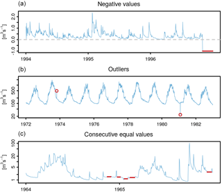
Figure 1 Three example time series illustrating issues detected by the three daily quality control criteria (highlighted in red). The first panel shows negative values at the end of the time series of Rohr at Rohrhardsberg, Germany. The second panel shows two outliers detected in the time series of Vakhsh at Gram, Tajikistan. The third panel shows instances of more than 10 consecutive equal values found in the time series of Tanara at Ponte di Nava, Italy. Note that all time series were trimmed for visualization purposes. Note also the logarithmic axis in panels two and three.

3 Streamflow indices

3.1 General considerations, design rules and reliability

3.1.1 General considerations

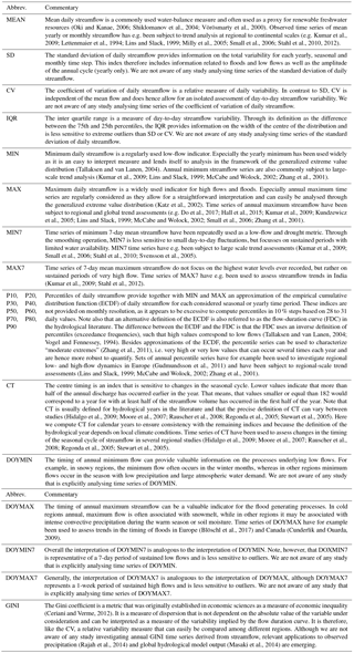
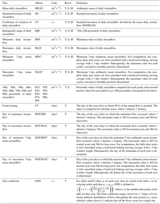
Table 3 describes a set of streamflow time-series indices that are designed to facilitate the analysis of (i) changes in the regional water balance, (ii) changes in the seasonal cycle, (iii) floods, and (iv) low flows. Many of the considered indices have been previously used in the scientific literature and Table 4 presents, wherever possible, a selection of relevant references and additional information. Note also that index selection was limited to those that can be computed without a base period, which excludes many; examples include “the number of days in a year, or season, for which daily values exceed a time-of-year-dependent threshold” (Zhang et al., 2005), drought deficit volumes (Loon and Anne, 2015; Tallaksen et al., 1997) and anomalies with respect to a climatological normal (McKee et al., 1993; Shukla and Wood, 2008). There are two reasons for excluding these indices: first, regional differences in temporal coverage hinder an unambiguous identification of a common base period that can be used around the globe. Second, it is now well established that indices that depend on a base period are prone to inhomogeneities if the base period is shorter than the considered series (Sippel et al., 2015; Zhang et al., 2005). Although both analytical (Sippel et al., 2015) and non-parametric (Zhang et al., 2005) solutions exist to mitigate this problem, we chose not to include indices that require a base period. This is because the available solutions either depend on strong normality assumptions (Sippel et al., 2015) or are computationally intensive (Zhang et al., 2005), which implies that the time-series indices cannot be easily extended when new data become available. Finally, it is noteworthy to mention that indices are easier to update when they do not have a base period, as they can be computed without knowledge of previous values.

Table 3 Definition of time-series indices contributing to the GSIM archive. Abbrev. Indicates the abbreviation of the index name used throughout this paper as well as in the database. Resol. indicates the time resolution for which the index is computed, which can take values of Y (yearly), seasonal (S) and monthly (M).

Table 4 Commentary and literature supporting the GSIM indices.

3.1.2 Design rules for index calculation

The design rules for calculating time-series indices closely follow the recommendations of ECA&D13. Before index calculation, all daily values that are flagged as suspect by the daily QC procedure are set to missing, and indices are computed using the remaining data points. All indices are computed on yearly time steps, while some indices are also computed with seasonal and monthly resolution. Seasons are defined as December–January–February (DJF), March–April–May (MAM), June–July–August (JJA) and September–October–November (SON). The reason for not computing all indices for seasonal and monthly resolutions is related either to the fact that some indices are only defined on annual timescales, or to the amount of data required for reliable computation. All considered indices are described in Tables 3 and 4.

3.1.3 Reliability of index values

Not all daily time steps have observations, and some daily observations have been flagged as suspect and were therefore removed. Consequently yearly, seasonal and monthly index values are not equally reliable. To allow users to judge the reliability of index values at individual time steps, the number of daily values used for index calculation at each time step is provided. Based on the recommendations of ECA&D13, the following rules for daily data availability can be applied to identify reliable index values.

1. Index values at a yearly time step are reliable if at least 350 daily observations are declared reliable.

2. Index values at a seasonal time step are reliable if at least 85 daily observations are declared reliable.

3. Index values at a monthly time step are reliable if at least 25 daily observations are declared reliable.

Note, however, that these are very conservative rules which may be relaxed depending on the needs of specific applications.

3.2 Example time series

To provide a first impression of the considered indices, Fig. 2 shows all indices at annual resolution for Wiese at Zell, located in south-western Germany. In addition, Fig. 3 shows the MEAN at monthly, seasonal and yearly resolutions of the same river.

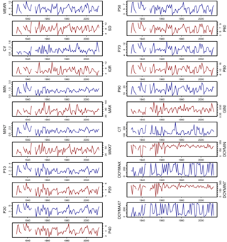
Figure 2 All considered indices at yearly resolution, shown for the River Wiese at Zell, south-western Germany. Yearly values are only displayed if they contain at least 350 reliable daily observations. See the text for details on units, interpretation and reliability classification.

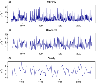
Figure 3 Monthly, seasonal, and yearly MEAN for the River Wiese at Zell, south-western Germany. Index values are only displayed if they fulfil the ECA&D13 data availability criteria. See the text for details.

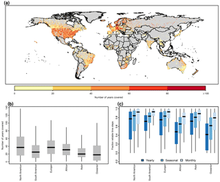
Figure 4 Temporal coverage of streamflow time-series indices. (a) Map of the number of years covered by each time series under consideration. (b) Distribution of the number of years available per time series for the continental regions of the world. (c) Distribution of the fraction of time steps that are classified as reliable using the ECA&D13 data availability criteria. Boxplots show the interquartile range (box) and the median (vertical bar); the whiskers extend to the most extreme point, which is not more than 1.5 times the interquartile range away from the box; outliers are omitted.

3.3 Temporal coverage of yearly, seasonal and annual indices

Figure 4a displays the number of years covered by all considered time series, highlighting both large variations in station density and time-series length, which is consistent with the availability of the original daily time series (Do et al., 2018a). To better appraise regional differences in temporal coverage, Fig. 4b shows the distribution of the number of years that are typically available for each station for major continental regions. The median time-series length is longest for North America and Europe and shortest for Oceania and Asia. The above-mentioned daily quality control (Sect. 2) as well as ECA&D13 criteria for judging the reliability of yearly, seasonal or monthly index values (Sect. 3.1.3) imply that the space–time coverage of the index data is not equal to the coverage of the original daily time series. Figure 4c shows the distribution of the fraction of time steps that were classified as reliable for the considered continental regions and for yearly, seasonal and monthly resolutions. Overall the figure highlights that the fraction of reliable time steps is largest for the Americas, Europe and Asia, while it is lowest for Oceania and Africa. Furthermore, it should be noted that the fraction of reliable time steps is lowest for yearly indices. This is related to the fact that full years are deemed unreliable when fewer than 350 valid observations are used for computation (following the ECA&D13 rules). Note however that the relatively strict ECA&D13 rules can be relaxed and should be adapted depending on user needs.

4 Homogeneity assessment

4.1 Methods for homogeneity assessment

4.1.1 Homogeneity tests

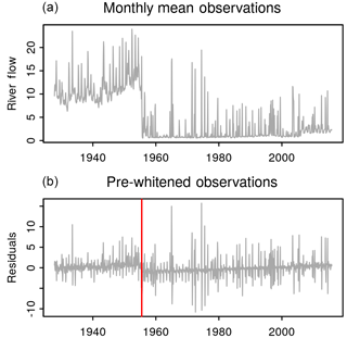
Figure 5 Homogeneity assessment of monthly mean flow of the North Umpqua River, US. (a) Monthly mean observations. (b) Pre-whitened observations together with the time step at which the standard normal homogeneity test, the Buishand range test and the Pettitt test identified a breakpoint at the 0.01 significance level.

Any environmental time series can be subject to inhomogeneities, i.e. unnatural sudden shifts in their statistical moments. In the simplest case, such inhomogeneities could be a jump in the mean between two time periods (see Fig. 5, top), but also changes in variability (e.g. reduced peak flows) or shifts in higher-order moments. The reasons for such inhomogeneities in streamflow time series are manifold, but they can “be related to changes in instrumentation, gauge restoration, recalibration of rating curves, flow regulation or channel engineering” (Gudmundsson and Seneviratne, 2016). As all the above-mentioned factors can be detrimental to a scientific investigation, it is essential to check time series against inhomogeneities. Here we apply a previously utilized collection of tests (Gudmundsson and Seneviratne, 2016), which is recommended by ECA&D13 and has been thoroughly tested for temperature and precipitation indices (Wijngaard et al., 2003). This collection of tests contains (i) the standard normal homogeneity test (Alexandersson, 1986), (ii) the Buishand range test (Buishand, 1982), (iii) the Pettitt test (Pettitt, 1979), and (iv) the von Neumann ratio test (von Neumann, 1941). For the application of the above-mentioned collection of tests, we rely on tables that provide critical values of the test statistics for a given sample size that have been determined using Monte Carlo methods (ECA&D13). These tables only report critical values for a sample size of 20 and larger. Therefore, the tests can only be applied if at least 20 yearly, monthly or seasonal time steps are available. Prior to homogeneity testing, yearly, seasonal and monthly index values that are classified as unreliable according to ECA&D13 (see Sect. 3.1.3) are set to missing. Missing values were removed after pre-whitening of yearly, seasonal and monthly index time series (see Sect. 4.1.2).

4.1.2 Pre-whitening

As the considered homogeneity tests rely at least on the assumption that the data are stationary, independent and identically distributed, all indices are pre-processed (pre-whitened), aiming to reduce effects of (i) trends, (ii) seasonality, and (iii) serial correlation. For the pre-whitening procedure, linear trends and mean seasonal cycles were removed using a linear least-squares regression model which captures both the trend and the mean values as $x=b+at$, where b is the intercept, a is the trend and t is time.

1. For yearly indices, the linear model is fitted to and subtracted from the complete time series. This results in a time series with zero mean and no linear trend.

2. For seasonal indices, the linear model is fitted to and subtracted from the time series for each season (DJF, MAM, JJA, SON) individually. This results in a time series with seasonal resolution in which each season has a zero mean and no linear trend.

3. For monthly indices, the linear model is fitted to and extracted from the time series for each month (January, February, etc.) individually. This results in time series with monthly resolution in which each month has a zero mean and no linear trend.

As the detrended and de-seasonalized time series may still exhibit serial correlation, they were further pre-whitened by fitting a lag-1 autoregressive model and then obtaining the residuals, which are then subjected to the homogeneity analysis (Burn and Elnur, 2002; Chu et al., 2013; Gudmundsson and Seneviratne, 2016). The lag-1 autoregressive model is fitted using maximum likelihood estimation.

4.1.3 Classification of station homogeneity

To effectively combine the information of the four considered homogeneity tests, we classify the homogeneity of yearly, monthly and seasonal time-series indices following recommendations of ECA&D13:

1. useful: one or no tests reject the null hypothesis at the 1 % level;

2. doubtful: two tests reject the null hypothesis at the 1 % level;

3. suspect: three or four tests reject the null hypothesis at the 1 % level.

Note, however, that depending on the application, these rules may be either too relaxed or too conservative. In addition, we also introduce the following categories to account for special circumstances that can occur in this large-scale application:

• 4.

  not sufficient data: less than 20 yearly, seasonal or monthly reliable index values are available;

• 5.

  constant: all yearly, seasonal or monthly time steps have the same value;

• 6.

  error: an error (e.g. numerical convergence issue) occurred at any processing step.

4.2 Homogeneity testing of all yearly, seasonal and monthly time-series indices

The homogeneity analysis is applied to all indices at yearly, seasonal and monthly resolution. The rationale for applying the four tests to all indices individually is that inhomogeneities at a particular location might be relevant only for a subset of indices, while other indices are not affected. For example, it is possible that a change in instrumentation will affect peak flows, while low flows are not affected. For this homogeneity assessment, all yearly, seasonal and monthly time steps that are classified as reliable (Sect. 3.1.3) are considered. This results in a conservative assessment as (i) strict data-availability criteria are applied, and (ii) because inhomogeneities could occur in a time window not relevant to a study. Therefore, the presented results can be used for a general overview of time-series homogeneity, but their suitability should always be re-considered prior to specific applications.

Figure 5 illustrates the results of the homogeneity assessment for the MEAN index for the North Umpqua River in the US. The top panel shows the monthly MEAN index, which displays a sudden jump after the first third of the record. This jump may for example be the result of upstream flow regulation and would be detrimental for climatological investigations. The lower panel shows the time series after the above-mentioned pre-whitening procedure was applied. The seasonal cycle is effectively removed and obtaining the residuals from the lag-1 autoregressive model reduced the magnitude of the sudden jump. Note also the spurious trend, which is an artefact of the de-trending that occurs in the presence of strong, sudden shifts in the mean. Nevertheless, three of the four considered tests identify this inhomogeneity at the 0.01 significance level, and the series is classified as suspect.

Global summaries of the number of stations in different homogeneity classes are shown in Fig. 6. Owing to the reduced number of time steps, the homogeneity testing could only be applied for approximately half of the locations at yearly resolution. Nevertheless, the homogeneity assessment highlights that the other half of the yearly indices can be considered “useful” at many locations. Only a small number of the low-flow indices (e.g. MIN, P10, P20, P30) had “constant” values and other issues were rarely detected. For both seasonal and monthly resolution, the number of stations with sufficient data for homogeneity assessment increased significantly, although it is important to recall that the homogeneity tests were in many cases applied to relatively short records (i.e. at least 20 seasons or 20 months respectively). Most of the seasonal and monthly time series with sufficient data are classified as “useful”, but a number of “doubtful” and “suspect” values were also detected. At a few locations, low-flow indices had constant values.

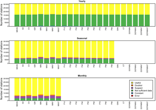
Figure 6 Global summary of the homogeneity analysis for all considered indices at yearly, seasonal and monthly resolution. Shown are the number of stations that are classified as (1) useful, (2) doubtful, (3) suspect, (4) not sufficient data, (5) constant and (6) error according to Sect. 4.1.3. Note that all six categories do occur, although some of them are rare and thus barely visible in the figure.

Figure 7 Continental summary of the homogeneity analysis for yearly, seasonal and monthly indices. Shown are the total number of stations at which all indices are classified as useful according to the criteria of ECA&D13, stations that did not have sufficient data for the application of the homogeneity analysis, and all other stations (other categories).

Figure 7 shows continental summaries of the homogeneity assessment at yearly, seasonal and monthly timescales and highlights the number of stations at which all indices were classified as useful according to the ECA&D13 criteria. Interestingly, the fraction of time series for which all indices have been classified as “useful” remains approximately constant irrespective of the considered time resolution. Figure 8 illustrates the effect of data availability criteria (Sect. 3.1.3) and the homogeneity assessment of the number of stations for each time step. Regardless of the temporal resolution, the number of stations reduces significantly when the homogeneity criterion is applied. This effect is more prominent at finer temporal resolution (monthly), as adding the “all indices homogenous” criterion removes approximately half of the eligible time series (bottom panel of Fig. 8). Note, however, that the presented summaries can only act as a rough guide on data availability, as criteria for including or excluding specific stations will depend on the objectives of individual future assessments.

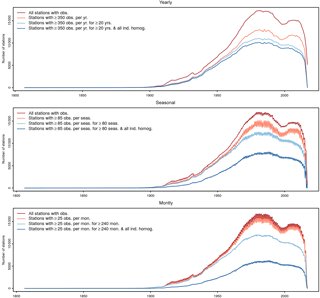
Figure 8 Temporal evolution of global station coverage, conditional on different data-selection criteria for yearly, monthly and seasonal timescales. Successively, the following criteria are applied: (i) all stations that at least one observation for the respective time step (i.e. year, season, month). (ii) Stations that have at least a critical number of observations for each time step (critical values depend on the timescale; see Sect. 3.1.3). (iii) Stations that have at least a critical number of observations for the equivalent of 20 station years (i.e. 20 yearly values, $\mathrm{20}\times \mathrm{4}=\mathrm{80}$ seasonal values, $\mathrm{20}\times \mathrm{12}=\mathrm{240}$ monthly values). (iv) Stations where criterion (iii) applied and all indices were considered to be useful in the homogeneity analysis (see Sect. 4.1.3).

5 Data availability and overview of the data product

5 Data availability

The data described in this paper are freely available as a compressed zip archive that can be downloaded from https://doi.pangaea.de/10.1594/PANGAEA.887470 (Gudmundsson et al., 2018). The zip archive contains (i) a readme file, (ii) all time-series indices and (iii) the results of all homogeneity tests. Note that the data are accompanied by additional information on the data collection process, catchment boundaries and selected catchment properties (Do et al., 2018a, b).

5.2 Time series of yearly, seasonal and annual indices

The indices derived from daily streamflow time series as described in Sects. 2 and 3 are stored in the INDICES directory. To address the different temporal resolution of the available indices (yearly, seasonal and monthly scales), the GSIM indices were organized into three respective subdirectories where each GSIM station is represented through a text file. For instance, indices at yearly resolution derived from the station with the identifier “AR_0000006” are stored as a text file called “AR_0000006.year” in the “yearly” sub-directory. Indices at seasonal and monthly resolution are stored as “AR_0000006.seas” and “AR_0000006.mon” in the respective (“seasonal”, “monthly”) sub-directories.

An identical data structure was adopted across all time-series files, with basic metadata (e.g. station identifier, station name, river name) stored in the header, and all index time series written in subsequent lines as a table, where (i) the first column contains the date, which is by convention the last day of the respective yearly, seasonal or monthly time step; (ii) the subsequent columns contain the index values, with column names corresponding to the abbreviations introduced in Table 4; and (iii) the last two columns contain information on the number of (missing) daily values used to compute the index.

5.3 Homogeneity of time-series indices

The results of the homogeneity analysis are stored in three tables, representing indices at yearly, seasonal and monthly resolution which are placed in the HOMOGENEITY directory and contain information on all stations. There is an identical structure for these three text files, with the first 13 columns containing important metadata such as the station identifier, name of the gauging location, and first and last time steps of the index time series. The remaining columns contain the results of four homogeneity tests that are described in the paper, and thus each index is accompanied by four columns (corresponding to the results of the (1) standard normal homogeneity test, (2) the Buishand range test, (3) the Pettitt test and (4) the Neuman ratio test).

6 Summary and conclusions

Together with Do et al. (2018a) (Part 1), this paper presents the Global Streamflow Indices and Metadata Archive (GSIM), which is a unique collection of streamflow observations at more than 30 000 stations around the globe. In Part 1 (Do et al., 2018a) of the paper series we focussed on the collection and merging of freely available streamflow data worldwide. Part 1 also introduced shapefiles of catchment boundaries together with essential catchment properties such as land cover, topography and mean climatic conditions. As not all data providers allow for a free distribution of unprocessed daily values, we followed in Part 2 an approach that has been established through the ETCCDI in climate research (Klein Tank et al., 2009; Zhang et al., 2011) and introduced a set of time-series indices that can be used to assess the water balance, seasonality, low flows and floods, which are made freely available to serve the scientific community.

While focussing on time-series indices facilitates the re-distribution of the data, this approach inevitably comes with inherent limitations. For example, many applications, including hydrological or ecological modelling, may require daily resolution data and other studies may depend on indices not included in the presented collections. Consequently, some users may prefer to seek out the original data sources (see details in Do et al., 2018a) and access the raw daily streamflow values in that manner. Nevertheless, we would like to also highlight the advantages of time-series indices: a benefit of having pre-processed the daily streamflow data into indices is that they can be readily used in studies across large regions with minimal handling of raw data files. In addition, the selected indices foster a wide variety of assessments, including water balance calculations, extreme event analysis and the identifications of trends in the world's freshwater resources.

To ensure the reliability of the published data, we first evaluated the quality of individual daily values through a combination of quality flags developed by the data providers and a transparent numerical screening approach. Subsequently, the homogeneity of yearly, seasonal and monthly indices was assessed using reproducible methods, aiming at aiding potential users to gauge the suitability of individual time series for their research questions. Note, however, that it is not the intent of this project to derive a single “best” dataset, for example, by considering a pre-defined baseline period which gauges must cover, or by derivation of a so-called “high-quality” dataset by applying a rigorous set of quality criteria to available stations. While these approaches are of high value if a dataset is tailored to a specific application, the emphasis of GSIM is to provide a large database of streamflow observations by collating and standardizing many data sources around the world.

Given that data quality requirements can vary substantially, it will remain the work of individual users to establish selection criteria for each study, thereby finding a trade-off between data quantity (number of gauges) and data quality (record length, missing periods). While the criteria used to gauge the usability of the indices are based on the recommendations of ECA&D13, they necessarily rely on subjective decisions on what constitutes a “reliable index”. For example, in some climates a gauge may be “reliable” and yet unable to provide measurements for part of the year (e.g. seasonally dry or cold climates). For this reason, attempts have been made to provide flexibility, aiming at facilitating the user to judge upon “reliability” in the context of their applications. Nonetheless, it is our hope that enabling a wide usage of streamflow indices might also lead to greater scrutiny of the data, accumulated knowledge of performance of each site and improved methods for judging the quality of streamflow observations.

There are numerous unsettled scientific questions at the global scale that this dataset has the potential to support. For example, there are unresolved questions around the relationship between trends in rainfall extremes and hydrological extremes (Do et al., 2017; Westra et al., 2013), as well as developing a better understanding of the influence of human activities on the hydrological cycle more broadly (Barnett et al., 2008; Blöschl et al., 2017; Destouni et al., 2013; Gudmundsson et al., 2017; Hegerl et al., 2015; Jaramillo and Destouni, 2015). Expanding upon recent methodological developments (Gudmundsson and Seneviratne, 2015, 2016), the newly assembled data may act as a basis for developing gridded global-scale observation-based data products. There are also likely to be many applications in fields as diverse as hydro-ecology, water quality modelling, environmental assessment and socio-hydrology. We therefore expect the presented data to be a valuable source of information to answer pending questions in global freshwater research, e.g. in the context of the World Climate Research Program Grand Challenge on Water Availability (Trenberth and Asrar, 2014) or the international research efforts on “Change in hydrology and society” (Montanari et al., 2013).

The significant increase in global gauge density and record length through the GSIM archive would not have been possible without the fact that water agencies are increasingly making data accessible online. However, the benefits of this new collection are overshadowed by challenges that are essentially bureaucratic in nature: how to systematically collate, maintain and improve streamflow data globally and who should do it. While agencies such as the GRDC would provide a natural fit for this type of task, they are currently constrained in their capacity to commit to a regular and systematic upkeep of such a global dataset. This paper series represents a one-off initiative of the authors, requiring over a year's worth of checking and evaluation and with little to no capacity for updating or extending the dataset. While it is possible that updates might be achieved through similar future efforts from the community, they are likely to be ad hoc and far from ideal. There are many troubles that can result from patchwork efforts of data collating, including (i) orphaned versions that persist in usage despite updated data being available, (ii) gauges or regions becoming out-of-sync, (iii) repeated needs to identify duplicates in overlapping datasets, (iv) information loss between versions and poor upkeep of documentation, (v) competing or “forked” databases, and many more. To remedy this situation, the hydrological community needs to collectively improve the organization of initiatives for coordinated systems that facilitate updating, storage and documentation of existing data, and to lobby for existing closed databases to be made open and accessible. As part of a global imperative for improved streamflow data, there are a number of additional activities researchers might undertake. These include (i) providing new analyses that improve the quality and understanding of the existing database; (ii) developing new automated methods that can be used systematically to maintain or improve the quality of the instrumental record; (iii) providing additional streamflow observations from missing or currently inaccessible datasets; and (iv) deriving new observational data products though better ground-truthing of remote-sensed variables, reanalysis from hydrological models or upscaling of in situ observations using machine learning.