Wind waves in the North Atlantic from ship navigational radar: SeaVision development and its validation with the Spotter wave buoy and WaveWatch III

Wind waves play an important role in the climate system, modulating the energy exchange between the ocean and the atmosphere and effecting ocean mixing. However, existing ship-based observational networks of wind waves are still sparse, limiting therefore the possibilities of validating satellite missions and model simulations. In this paper we present data collected on three research cruises in the North Atlantic and Arctic in 2020 and 2021 and the SeaVision system for measuring wind wave characteristics over the open ocean with a standard marine navigation X-band radar. Simultaneously with the SeaVision wind wave characteristic measurements, we also collected data from the Spotter wave buoy at the same locations, and we ran the WaveWatch III model in a very high-resolution configuration over the observational domain. SeaVision measurements were validated against co-located Spotter wave buoy data and intercompared with the output of WaveWatch III simulations. Observations of the wind waves with the navigation X-band radar were found to be in good agreement with buoy data and model simulations with the best match for the wave propagation directions. Supporting datasets consist of significant wave heights, wave directions, wave periods and wave energy frequency spectra derived from both SeaVision and the Spotter buoy. All supporting data are available through the PANGAEA repository – https://doi.org/10.1594/PANGAEA.939620 (Gavrikov et al., 2021). The dataset can be further used for validation of satellite missions and regional wave model experiments. Our study shows the potential of ship navigation X-band radars (when assembled with SeaVision or similar systems) for the development of a new near-global observational network providing a much larger number of wind wave observations compared to e.g. Voluntary Observing Ship (VOS) data and research vessel campaigns.

1 Introduction

Ocean wind waves play a critically important role in air–sea energy and gas exchanges (Gulev and Hasse, 1998; Andreas et al., 2011; Blomquist et al., 2017; Ribas-Ribas et al., 2018; Cronin et al., 2019; Xu et al., 2021) and in ocean surface mixing (McWilliams and Fox-Kemper, 2013; Buckingham et al., 2019; Studholme et al., 2021), thus being an important active component of the coupled climate system (Cavaleri et al., 2012; Fan and Griffies, 2014). At the same time, massive long-term observations of wind waves over global oceans still have insufficient coverage and quality compared to other surface variables (e.g. air and sea surface temperatures). Wind waves are wind-driven ocean surface gravity waves. Visual wave observations from Voluntary Observing Ships (VOS), while providing the longest time coverage (formally going back to the mid-19th century), suffer from space- and time-dependent sampling biases as well as from both random and systematic biases and require continuous validation (Gulev et al., 2003). Remote sensing datasets of wind waves go back to 1985 (Ribal and Young, 2019), when the first satellite radar altimeter missions (Seasat in 1978 (the first satellite to provide data) and Geosat in 1985) were launched and started to provide ocean surface elevations with high temporal and spatial resolution. However, remote sensing data have to be validated against in situ measurements, typically available from buoys (such as NDBC buoys, Swail et al., 2010, or NOWPHAS, Nagai et al., 2005). Buoys measure vertical and horizontal displacements of the ocean surface (such as Spotter or Datawell buoys with up to 2.5 Hz sampling frequency, Raghukumar et al., 2019) and provide highly accurate estimates of wind wave characteristics, effectively now assimilated into Numerical Weather Prediction (NWP) models. Assimilation of the significant wave heights from wave buoys in operational wave models decreases root-mean-square error in significant wave height forecasts by 27 % on average (Smit et al., 2021). However, buoy networks are sparse, with most deployments being in the coastal regions, and can only effectively serve for verification of all other datasets rather than for developing global or regional climatologies.

Starting from the 1980s, considerable progress in wind wave modelling (WAMDI, 1988; Hasselmann et al., 1985; Cavaleri et al., 2020) resulted over the last decade in the development of multiple global and regional wind wave hindcasts generated by spectral wave models such as WAM (WAMDI, 1988) or WAVEWATCH (WW3DG, 2019) forced by atmospheric reanalyses or climate models, providing multidecadal wind wave fields with high temporal and spatial resolution (Casas-Prat et al., 2018; Semedo et al., 2018; Morim et al., 2020, 2022; Sharmar et al., 2021). Being currently a widely accepted source for estimating long-term climate variability in wave characteristics, wind wave hindcasts also suffer from the inaccuracy in the modelling of many aspects of wind wave dynamics, including e.g. extremely high wave peaks at high wind speeds during the storm passage (Cavaleri et al., 2020).

In summary, all three sources of global wind wave information (VOS, satellite data, and model hindcasts) require data for extensive validation. Existing wave buoys deployed in a few locations cannot solve this problem to the full extent. Thus, investigating alternative sources of massive wind wave data remains a challenge. In this respect, ship navigation radars represent an option whose potential, especially in open-ocean regions, is not yet explored to its fullest extent. Here, we present the results of the development and validation of the SeaVision system for wind wave observations in the open ocean using standard navigation marine X-band radars, which allows for real-time monitoring of wind wave characteristics along the commercial ship tracks.

Applicability of the navigation radars for measurements of the wind wave characteristics was first noted by Young et al. (1985). Radar images of the ocean surface, known as sea clutter, are generated by Bragg scattering (Crombie, 1955) of the electromagnetic signal by the ripples on the ocean surface produced by the wind. Being emitted from the radar, an electromagnetic signal reaches the ocean surface and further, is reflected by ripples on the ocean surface, and is received back by the radar antenna when the ocean surface is rough enough (i.e. ripples are developed). Under a wind speed of >3 m s⁻¹ and wave height of >0.5 m, the surface wave field becomes detectable on the radar image of the sea clutter (Hatten et al., 1998; Hessner and Hanson, 2010). Time sequences of these images are further analysed to estimate the wind wave characteristics. The associated retrieval procedures can be based on various approaches, which include a signal-to-noise ratio derived from the image spectrum (Nieto-Borge et al., 1999, 2008; Seemann et al., 1997), statistical analysis of the island-to-trough ratio in the sea clutter images (Buckley and Alter, 1997, 1998), analysis of the image texture (Gangeskar, 2000), the wavelet technique (An et al., 2015), the least square approach (Huang et al., 2014), and shadowing analysis (Gangeskar, 2014). Methodologies may also be based on the combination of these methods with the use of artificial neural networks (Vicen-Bueno et al., 2012). This may also include the analysis of the Doppler shift of the received radar signal that is based on the well-defined relationship between orbital velocities and wave height for linear gravity waves (Plant, 1997; Plant et al., 1987; Johnson et al., 2009; Karaev et al., 2008; Hwang et al., 2010; Story et al., 2011; Chen et al., 2019). There are many aspects of the sea clutter radar image analysis: Nieto-Borge and Guedes Soares (2000) for example proposed an approach considering superpositions of swell and wind sea components that allowed them to derive wind wave and swell contributions to the total wave field, along with directional characteristics. There are also attempts to use images of the sea clutter revealed from X-band radars for estimating the current-depth profiles with an Eulerian approach (Campana et al., 2017), to retrieve wind speed and wind direction (Chen et al., 2015; Dankert and Horstmann, 2007; Dankert et al., 2003; Vicen-Bueno et al., 2013) and to derive surface characteristics (Senet et al., 2001).

On this basis, several commercial systems such as WaMoS II (http://www.oceanwaves.de, last access: 2 August 2022), SeaDarQ (Greenwood et al., 2018), and WaveFinder (Park et al., 2006) were developed. The most widely used system nowadays is WaMoS II (software and hardware details provided in Reichert et al., 2006); it is focused on the operational monitoring of the sea state (wind wave and surface currents) and operational management of oil platforms and ships using nautical X-band radars. Derkani et al. (2021) provided a dataset of the wind, wave, and surface currents over the Southern Ocean collected with WaMoS II (Alberello et al., 2020c; Derkani et al., 2020).

In combination with other sources of the data (altimetric wave radar, vessel hydrodynamic simulator), wind wave estimates from navigational radar can be used to manage security of the offshore systems, assess ship fatigue due to mechanical environmental influence (Drouet et al., 2013), or predict ship rolling in real time (Hilmer and Thornhill, 2015).

We present the design and pre-processing methodology of the SeaVision system along with the dataset collected during three research cruises (Fig. 1). SeaVision was developed in collaboration between the Shirshov Institute of Oceanology of the Russian Academy of Sciences (IORAS, https://ocean.ru/, last access: 4 August 2022) and the Joint Stock Company “Marine Complexes and Systems” (“MC&S” J.S.C., https://www.mcs.ru/, last access: 4 August 2022). SeaVision is developed on the basis of the sea ice monitoring system with navigational marine radar – IceVision (https://ice.vision/en, last access: 4 August 2022). The pilot version of SeaVision was tested and validated on two North Atlantic cruises in 2020 and 2021 and on the Arctic cruise in 2021 (Fig. 1). The major advantage of the presented dataset is the provision of the co-located Spotter wave buoy data with SeaVision records at almost 50 locations and outputs of WaveWatch III (WW3) model experiments forced by ERA5 reanalysis (Hersbach et al., 2020) for the corresponding domains. We present in this study the SeaVision system and dataset of the measurements of the wind waves in the open ocean and their comprehensive analysis.

The paper is organized as follows. In Sect. 2 we provide details of the research cruises, technical specifications of the SeaVision system, data collection, and analysis principles, as well as the description of the WW3 model set-up. Section 3 presents the results of the analysis and validation of the SeaVision dataset against Spotter buoy data and the comparison to the WW3 model output. The concluding Sect. 4 summarizes the results and discusses the perspectives of the use of ship navigation radars for a massively enhanced collection of wind wave information in the open ocean.

2 Data collection and analysis

We provide definitions of all parameters included in the published dataset in Appendix C. For wind and wave directions, we use the meteorological convention implying that both wind and waves are coming from the specified direction (blow into compass).

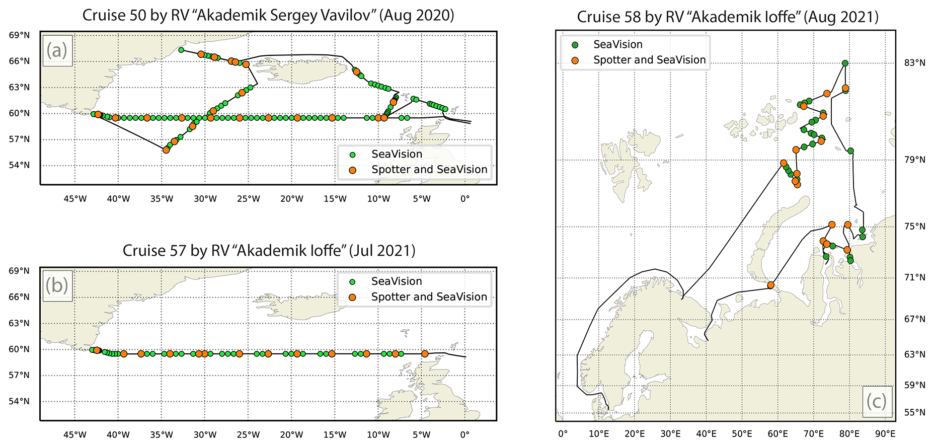
Figure 1 Ship tracks of the three cruises of the research vessels (R/Vs) Akademik Sergey Vavilov (a) and Akademik Ioffe (b, c). Green dots indicate locations where only SeaVision radar data were collected, and orange dots show the locations for which SeaVision records were co-located with Spotter wave buoy measurements. Cruise numbers are counted from the beginning of the R/V operation.

2.1 Ship cruises

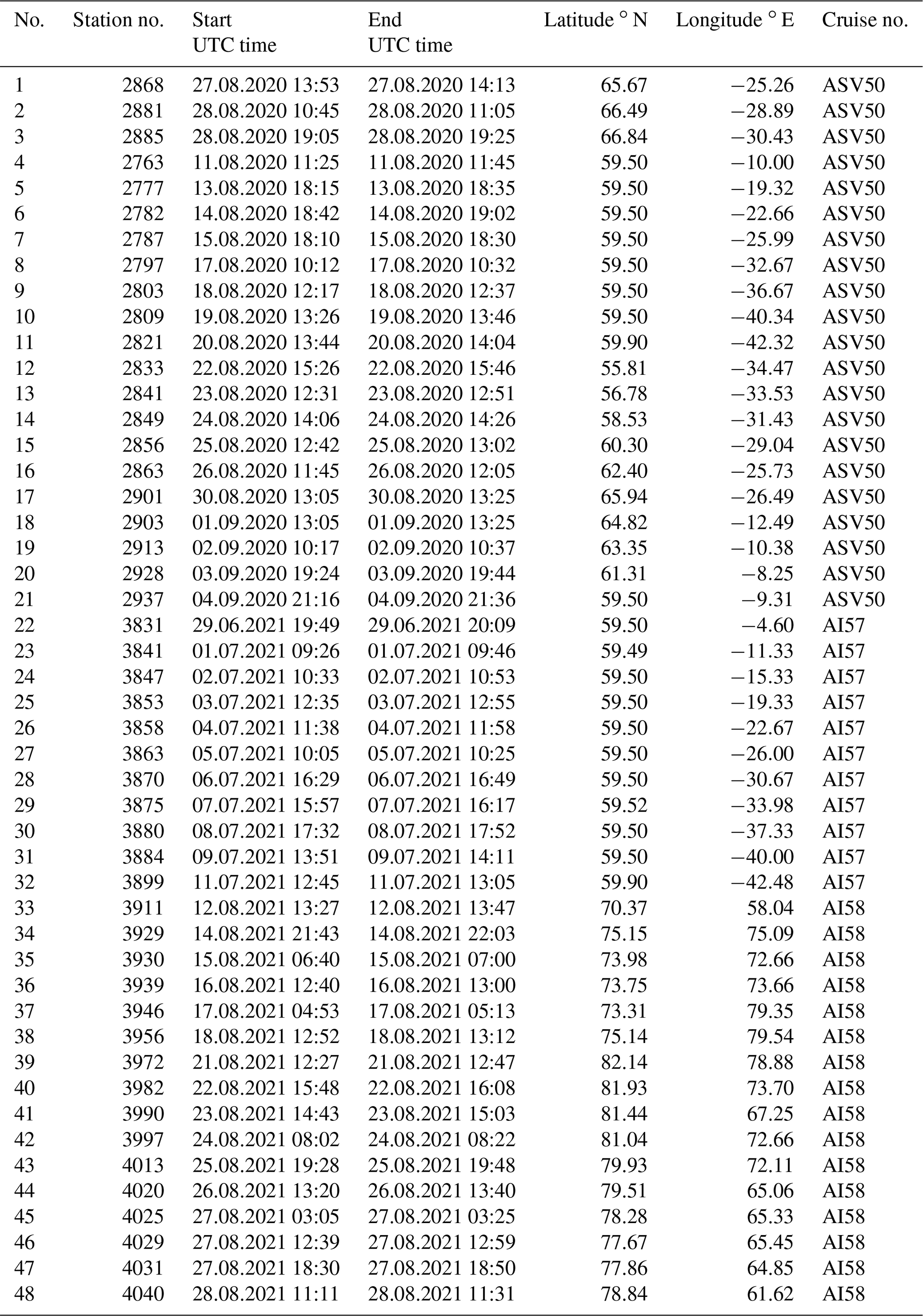
Figure 1 demonstrates ship tracks of the three research cruises, during which wind wave data were collected. Research cruises were carried out by IORAS research vessels (R/Vs) Academik Sergey Vavilov and Academik Ioffe. Table 1 provides general information about the cruises and detailed information on the coordinates and dates and is provided in Appendix A. The two cruises in the subpolar North Atlantic (Fig. 1a, b) were focused on the regular survey of the 59.5^∘ N oceanographic trans-Atlantic cross section and cross sections in the Denmark Strait (Verezemskaya et al., 2021). During these cruises the R/V does full-depth conductivity–temperature–depth (CTD) profiling. The distances between the hydrographic stations vary from ∼30 km in the open ocean to a few kilometres near the East Greenland coast, with the time allocated for each station (the ship is drifting) varying from 2 to 6 h. Here and later in the paper we determine stations as the locations where wind wave observations were carried out (Table A1). Between the stations the R/V travels at a speed of approximately 6 to 10 kn. During the cruise of R/V Academik Ioffe in the Kara Sea (Fig. 1c), stations were somewhat shorter in time (2–3 h). During all cruises wave observations were carried out after completing hydrographic profiling. For operating solely SeaVision, the R/V position was strictly stationary, being controlled by bow and stern thrusters of the R/V. When SeaVision was used together with the free-drifting Spotter buoy, the thrusters were off to also provide free drifting of the R/V. This allowed for measurements of the background wave field by both SeaVision and the Spotter buoy. At each station we first released the Spotter buoy with a supplementary floating buoy dumping cable vibrations. Such a design allows for the maintenance of at least 300 m distance between the buoys and the R/V. Then, both buoys were in the free-floating mode for at least 30 min, during which the recording was performed by both SeaVision and the Spotter buoy (Fig. 4a). Lastly, both buoys were pulled back on board. The Spotter buoy measured vertical and horizontal displacements, starting from its release until being retrieved back on board. After completing measurements at each station, only the data recorded during the free-floating mode were used for the joint analysis of SeaVision and Spotter buoy records. During all SeaVision and Spotter buoy measurements, standard meteorological parameters were measured using the onboard meteo station.

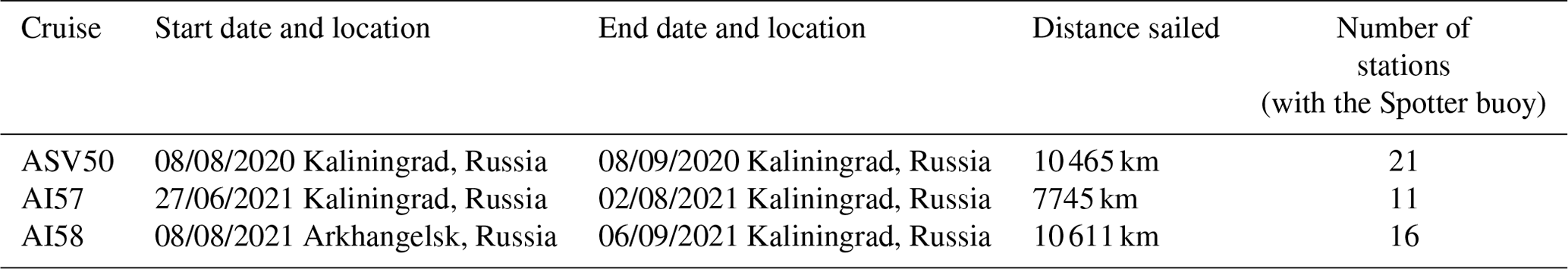
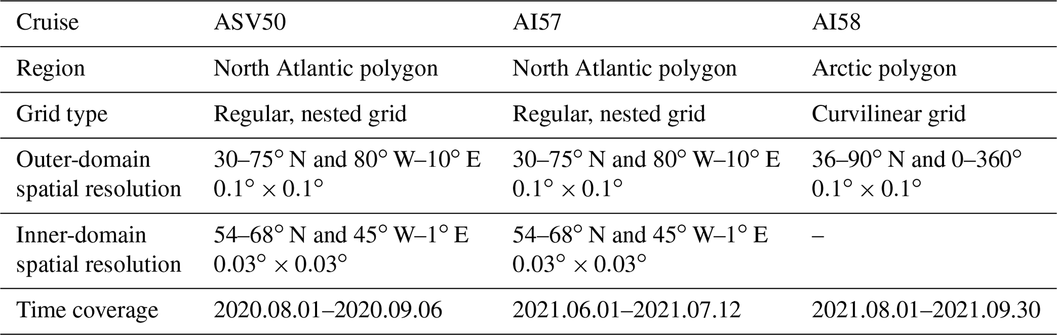
Table 1 Research cruises during which the wind wave observations were carried out by research vessels (R/Vs) Akademik Sergey Vavilov (ASV) and Academik Ioffe (AI). Adjacent numbers in the first column correspond to the R/V cruise numbers counted from the beginning of the R/V operation.

2.2 SeaVision system

2.2.1 Ship navigation radar signal retrieval and pre-processing

Development of the SeaVision system was based on a commonly accepted approach to the recording and analysis of the sea clutter images. Using a similar approach, commercial systems such as WaMoS II (http://www.oceanwaves.de, last access: 4 August 2022), SeaDarQ (Greenwood et al., 2018), and WaveFinder (Park et al., 2006) were developed. These commercial systems provide customers with their original software and hardware. In our approach we are focused on the development of an independently operating, low-cost, and easy-to-install system compatible with the existing ship navigation radars.

Research vessels Academik Sergey Vavilov (R/V ASV) and Akademik Ioffe (R/V AI) are equipped with the standard navigation X-band radars JRC JMA-9110-6XA and JMA-9122-6XA. Technical details of radar transmission and backscattering characteristics are given in Table 2. Both radars operate at 9.41 GHz frequency (wavelength ∼3 cm) and are equipped with a 6 ft antenna with a directional horizontal resolution of 1.2^∘ (Table 2). Radars can optionally operate at pulse lengths of 0.08, 0.25, 0.5, 0.8, and 1.0 µs. For our purposes we used the smallest possible pulse length of 0.08 µs (in the so-called “short-pulse” mode – SP1), providing the highest possible resolution of the image (and thus the best resolution of the ocean surface). Our X-band radars are characterized by a 3.18 cm wavelength of the emitted electromagnetic waves (Table 2). The pulse length is the emission time of the wave beam; thus, the number of the emitted waves and the area of reflection at the ocean surface (defining spatial resolution) increase with increasing pulse length.

The SeaVision system (Fig. 2) is connected to the radar via a splitter. It provides digitizations and further recording of the directionally stabilized (northward) radar sea clutter image resulting from each single full turn of the radar antenna. By doing this, SeaVision converts the sea clutter image into a digital format and records the data onto the external storage. SeaVision is also connected to the ship navigation package and simultaneously records geographical coordinates from GPS, speed over ground (SOG), and course over ground (COG). Each full turn of the antenna results in an ASCII file (∼16 MB) consisting of a 4096×4096 matrix (1.875 m discretization at 4096 beam directions) representing the sea clutter digitized image with GPS information, SOG, and COG in the file header. These files are further consolidated and converted into NetCDF format at the post-processing stage.

Table 2 JRC JMA-9110-6XA radar (R/V ASV) and JMA-9122-6XA (R/V AI) transmission and reception characteristics.

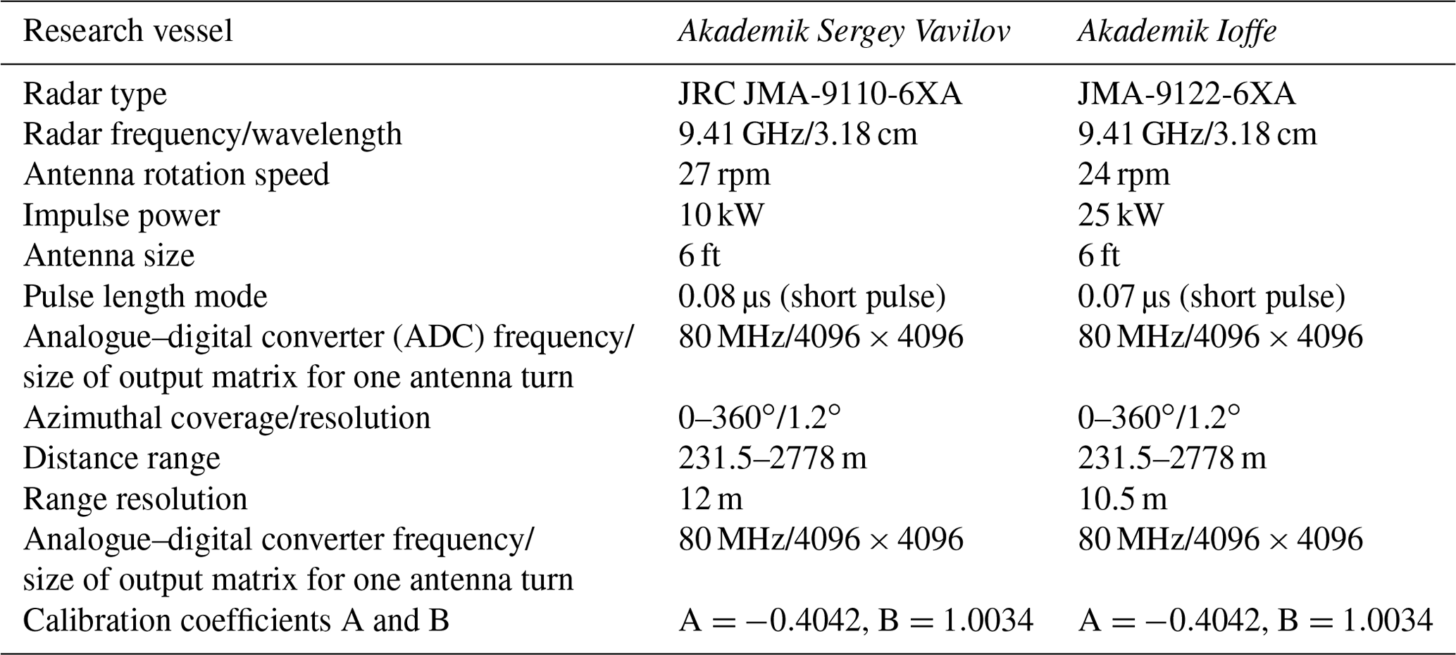
Figure 2 SeaVision integration to the ship's navigational equipment together with an example of the series of the geographically stabilized (northward) sea clutter images, one for each antenna turn (right column). The image of the JRC radar scanner (top left) is taken from http://www.jrc.co.jp/eng/index.html (last access: 4 August 2022).

2.2.2 Analysis of the sea clutter images

After the sea clutter images are collected and digitized, the next step is the post-processing focused on the computation of significant wave height (H_s), wave period (T_m01), wave energy spectrum (S_w), and wave direction (D_s). Here we provide a short condensed description of the algorithm, with the full details given in Appendix B. The subset collected at each station (Fig. 1) consists of the 20 min SeaVision record, which is equivalent to at least 540 images of the sea clutter (27 antenna full turns per minute for the JRC JMA-9110-6XA radar).

The methodology for estimation of wind wave characteristics relies on a well-established Fourier transform (FT) technique (Nieto-Borge and Guedes Soares, 2000; Nieto-Borge et al., 2006). For each station, pre-processing of the data begins with the choice of the processing squared area (squared area of 720×720 m). For now, we locate the processing area visually by taking the area of the most apparent wave signal in the image and requiring this area to be distanced from the ship by 300 m to avoid a potential impact of the ship on the wave field and the effects of the reflection and modulation of the radar signal by the ship superstructure. When the processing area is selected, we consolidate the data captured in this area from all 540 images for further analysis. Note that the data initially sampled in polar coordinates are re-gridded at this step to a Cartesian grid of 384×384 grid points with 1.875 m spatial resolution for each subset.

The sequence of 540 matrices with 384×384 grid points each is then split into 16 sectors (22.5^∘ width each). Further, to obtain the directional spectrum estimates, we transformed the data into a 3D spectral domain by using the Fourier transform and applying the Welsh method with a half-width overlapping Hanning window (48 points, Fig. 3). This returns, for each sector, the 3D spectrum S_3d,image (k_xk_yf), where $f=\mathit{\omega }/\mathrm{2}\mathit{\pi }$ is the frequency (Hz) and ω is the angular frequency, and k_x and k_y (rad m⁻¹) are the components of the wave vector k(k_x,k_y). Then, for each sector we capture the spectrum power within the band along the line satisfying the linear dispersion relation for ocean waves (Fig. 3):

$$\begin{array}{}\text{(1)}& \mathit{\omega }=\sqrt{gk}+kU\cos \mathit{\theta },\end{array}$$

where k is the wavenumber (rad m⁻¹), g is gravity (m s⁻²), U is the surface velocity (m s⁻¹) which includes surface current velocity and ship drift, and θ is the angle between the wave vector k and velocity vector U. This procedure is applied to the bands corresponding to the first and second spectral harmonics (see Appendix B for the definition of band width). The spectral power outside the bands for the two harmonics is assumed to be a background speckle noise (ω_speckle) (Kanevsky, 2009). Integrated spectral power outside of the bands matching the wave dispersion relation Eq. (1) is further used to estimate the signal-to-noise ratio (SNR) as described in Appendix B and outlined in many works (Nieto-Borge et al., 1999; Hessner et al., 2001; Young et al., 1985; Nieto-Borge and Guedes Soares, 2000; Ivonin et al., 2016). Following Nieto-Borge et al. (1999, 2006), the SNR is then converted to significant wave height H_s,SeaVision using the linear regression equation:

$$\begin{array}{}\text{(2)}& H_{\mathrm{s},\mathrm{SeaVision}}=A+B\sqrt{\mathrm{SNR}},\end{array}$$

where A and B are empirical calibration coefficients which are specific to each radar. In this study, these coefficients were computed by fitting a linear regression Eq. (2) to the significant wave height measured by the Spotter wave buoy. Derived numerical values of A and B coefficients are given in Table 2 for both X-band radars. Wave period T_{m01,SeaVision} was estimated conventionally using the zeroth and first spectral moments:

$$\begin{array}{}\text{(3)}& {\displaystyle }{T}_{\mathrm{m}\mathrm{01},\mathrm{SeaVision}}={\displaystyle \frac{m_{\mathrm{0},\mathrm{SeaVision}}}{m_{\mathrm{1},\mathrm{SeaVision}}}},\text{(4)}& {\displaystyle }{\mathrm{m}}_{\mathrm{0},\mathrm{SeaVision}}={\int }_{\mathrm{0}}^{\mathrm{\infty }}{S}_{\mathrm{w},\mathrm{SeaVision}}\left(f\right)\mathrm{d}f,\text{(5)}& {\displaystyle }{\mathrm{m}}_{\mathrm{1},\mathrm{SeaVision}}={\int }_{\mathrm{0}}^{\mathrm{\infty }}{S}_{\mathrm{w},\mathrm{SeaVision}}\left(f\right)f\mathrm{d}f,\end{array}$$

where S_w,SeaVision(f) is the estimate of the wave energy spectrum from SeaVision,

$$\begin{array}{}\text{(6)}& S_{\mathrm{w},\mathrm{SeaVision}}\left(f\right)={\left({\displaystyle \frac{{\mathrm{H}}_{\mathrm{s},\mathrm{SeaVision}}}{{\mathrm{H}}_{\mathrm{s},\mathrm{image}}}}\right)}^{\mathrm{2}}{\mathrm{S}}_{\mathrm{image}}\left(f\right),\end{array}$$

and H_s,image is $H_{\mathrm{s},\mathrm{image}}=\mathrm{4}\sqrt{m_{\mathrm{0},\mathrm{image}}}$, thus being the estimate of significant wave height using the raw sea clutter image before calibration.

We note that local weather conditions, specifically rain events, can potentially affect the electromagnetic radar signal as the raindrops absorb and scatter the radar signal. However, the analysis of current weather has shown that no rain events were observed during observations.

Figure 3 Organigram of the data processing for estimation of wind wave parameters from the sea clutter images. JRC radar scanner (top left) is taken from http://www.jrc.co.jp/eng/index.html (last access: 4 August 2022).

2.3 Spotter wave buoy data

To calibrate and validate SeaVision wave observations, we performed simultaneous measurements with the Spotter wave buoy (https://www.sofarocean.com/products/spotter, last access: 4 August 2022) in the locations shown in Fig. 1 and specified in Table A1. Once the ship was drifting at the locations of the measurements, the Spotter buoy was deployed and started drifting away from the ship. Note that the ship drift is always faster compared to that of the buoy; thus, the distance between the buoy and the ship progressively increases. When the distance between the ship and the buoy reached at least 300 m, the “free-floating” mode of SeaVision and Spotter buoy operation was initiated for at least 30 min as described in Sect. 2.1. The longest free-floating-mode time period at some stations reached up to 1.5 h. To ensure homogeneity of the analysis, we used 20 min segments from the “free-floating”-mode time series for further computations of significant wave height, wave spectra, and directional moments: $H_{\mathrm{s}}=\mathrm{4}\sqrt{E}$, where $E={\int }_{\mathrm{0.01}\mathrm{Hz}}^{\mathrm{1.25}\mathrm{Hz}}E\left(f\right)\mathrm{d}f$ – the surface elevation variance in the frequency range of the wind waves. Further, we used wave parameters derived from the Spotter buoy as a “ground truth” for the calibration of SeaVision data and derivation of A and B calibration coefficients in Eq. (2) (Table 2). An example of the wave energy spectrum for the 20 min Spotter buoy record is shown in Fig. 4b.

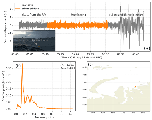
Figure 4 Spotter wave buoy time series of vertical displacements at station no. 3946 in the AI58 cruise (a), corresponding wave energy spectrum (b), and location of station no. 3946 (c).

2.4 Meteorological data

During all cruises, AIRMAR WeatherStation 220WX was installed on the main ship mast at 30 m height above the sea. The weather station provided an output consisting of standard output parameters (barometric pressure, wind speed and direction, air temperature, and relative humidity). Wind characteristics were recalculated from the relative wind to the true wind in real-time mode.

2.5 WaveWatch III model experiment

We ran the WaveWatch III (WW3DG, version 6.07, WW3) spectral wave model forced by ERA5 reanalysis (Hersbach et al., 2020) over the domain and the time period of the research cruises (Table 3). The experiments were performed for the outer domain at 0.1^∘ spatial and 1 h temporal resolution and for the inner domain with 0.03^∘ (∼1 km) spatial (see Table 3) and 1 h temporal resolution. The outer domain solution was used for setting lateral boundary conditions for the inner domain. These experiments returned 2D wave spectra co-located with SeaVision and Spotter buoy observations. In the WW3 experiments we used the ST6 parameterization (Bababin, 2006, 2011; Rogers et al., 2012; Zieger et al., 2015) for wave energy input and dissipation and the discrete interaction approximation (DIA) scheme for non-linear wave interactions (Hasselmann, 1985).

Table 3 WW3 model configuration over the domains of expeditions.

3 Results of validation of SeaVision measurements

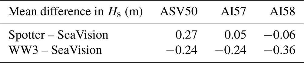
Validation of SeaVision data was provided for wind speeds from 2 to approximately 20 m s⁻¹ and for significant wave heights from a few tens of centimetres to 4.2 m. Figure 5 demonstrates the results of the intercomparison of significant wave height (H_s) estimates retrieved from SeaVision data and those measured by the Spotter buoy and simulated with WaveWatch III. The H_s differences “Spotter minus SeaVision” (Fig. 5a) and “WW3 minus SeaVision” (Fig. 5b) are plotted as a function of wind speed recorded by the ship's weather station (Table A1). Table 4 provides comparative estimates of differences in H_s for the three cruises. On average, WW3 yields lower wave heights than SeaVision H_s by 28 cm, while the agreement between SeaVision and the Spotter buoy data is better, with H_s measured by Spotter being around 10 cm higher than that retrieved from SeaVision. For low wind speeds SeaVision tends to underestimate H_s by up to 60 cm, and for moderate and strong winds the analysis shows an overestimation of SeaVision H_s compared to buoy and model data. This can be explained by better-developed ripples (affecting the signal-to-noise ratio) at the ocean surface under stronger winds.

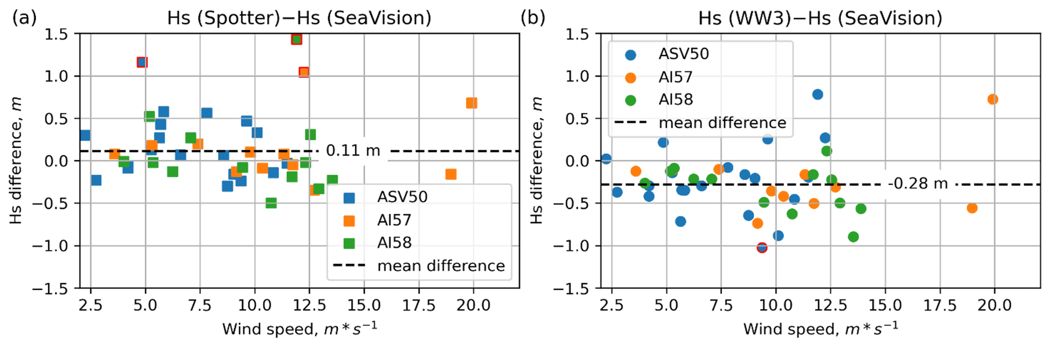
Figure 5 Difference in the significant wave height (H_s) estimates for all stations as a function of the wind speed: Spotter buoy (“ground truth”) minus SeaVision (a); WW3 minus SeaVision (b). Dash lines mark the mean difference across all data points. Red squares and circles mark differences higher than 1 m.

We also identified three locations (2901, 2928, and 2937; see Table A1) for which the differences between the Spotter buoy data and SeaVision reach more than 1 m (for 5 and 13 m s⁻¹ winds). Weather conditions for these cases were not associated with severe weather and H_s values were in the range between 1.5 and 2 m. However, in these cases we recorded a strong drift of the vessel due to the local current that potentially impacted the angle of the electromagnetic signal reflection from the surface and hence affected the accuracy of the radar images. Thus, strong ship drift may influence the SeaVision results, and the data collected under strong ship drift should be considered with caution. These cases, in the future, can be identified by analysis of speed over ground (SOG parameter). For “WW3 minus SeaVision” there is only one station, no. 2841, where this difference reaches 1 m.

Table 4 Differences in significant wave height estimates for the three cruises.

Scatterplots for the H_s and wave period (T_m01) demonstrate generally better agreement between different data sources for H_s (1.06 and 1.02 regression coefficients) than for T_m01 (1.05 and 0.86 regression coefficients) (Fig. 6). There is no robust evidence of the dependence of the magnitude or sign of H_s and T_m01 differences on the magnitudes of the parameters themselves. We also note that both SeaVision and Spotter show higher waves and slightly longer periods compared to WW3 (Fig. 6). We note, however, that simulated wind waves with WW3 strongly depend on the atmospheric forcing (choice of reanalysis). Difference in climatological mean values over the North Atlantic obtained with WW3 but with different forcing functions can reach a few tens of centimetres (Sharmar et al., 2021).

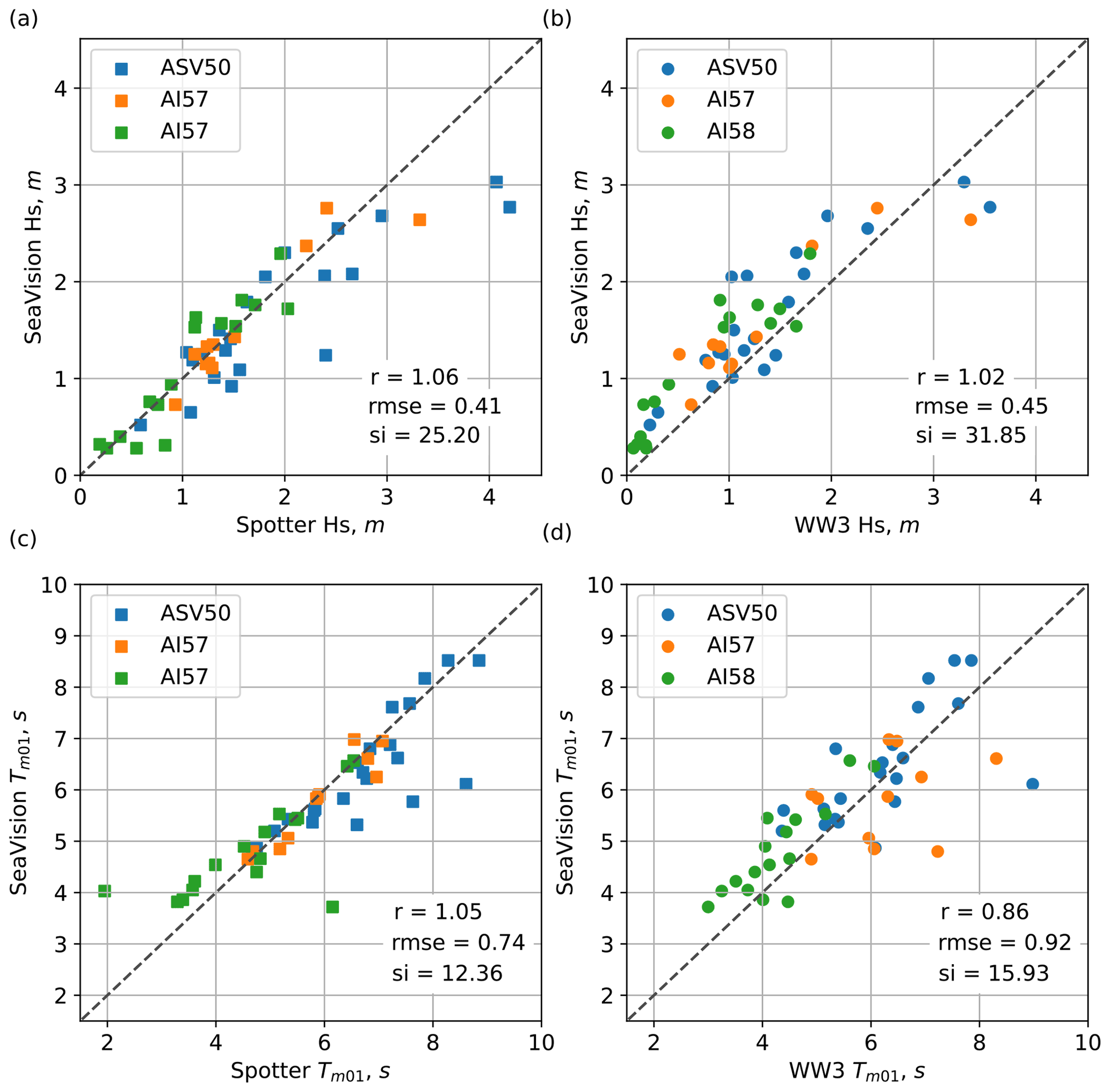
Figure 6 Scatterplots of the significant wave height (H_s) and wave period (T_m01) revealed by SeaVision and measured by Spotter (a, c) as well as revealed by SeaVision and simulated with WaveWatch III (WW3, b, d) for all stations, together with root mean square error (RMSE) and scatter index (SI) statistics.

Overall, the analysis of significant wave heights among these three sources of data (Spotter, SeaVision, and WW3) shows that the highest H_s values are measured by the Spotter buoy and the lowest simulated by WW3, with SeaVision being in between. These results are intuitively correct as wave buoys measure the actual elevations of the ocean surface, and SeaVision provides a proxy of local wave conditions from image analysis (thus imposing averaging over the domain) and is not expected to be as accurate as wave buoy data.

Figure 7 shows comparisons of wave directions (D_s) along with corresponding significant wave height (H_s) values (simplified approximation of directional spectra) for six stations (see Table A1). Generally, all three data sources demonstrate very good agreement on directions (differences in wave direction do not exceed 10^∘), with corresponding wave height estimates being underestimated in model simulations as already mentioned above (Figs. 5 and 6).

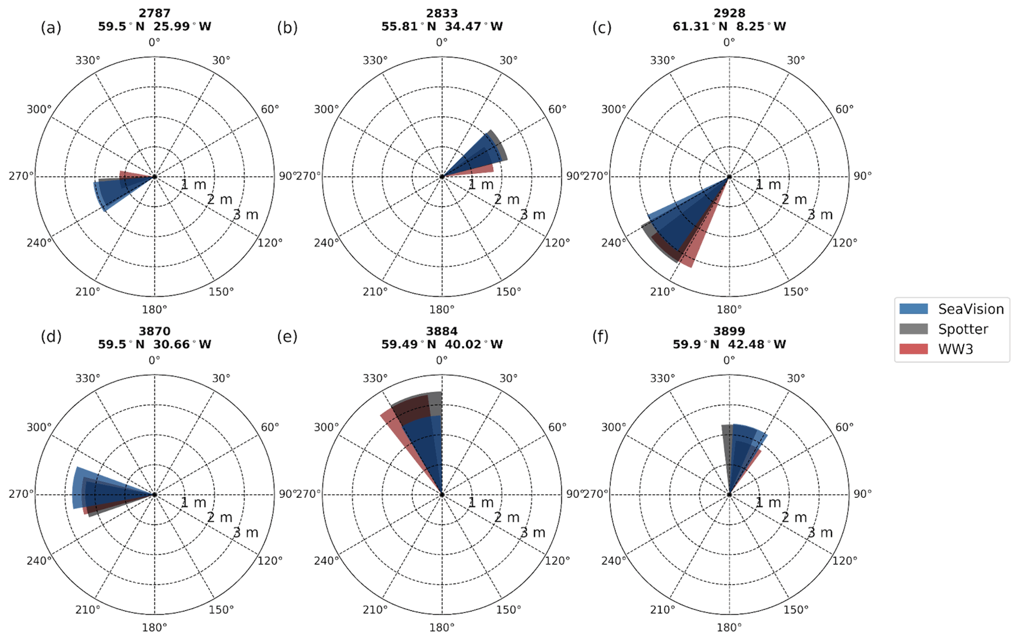
Figure 7 Diagrams (roses) of mean wave direction (D_s, from) and significant wave height (H_s) on the basis of the three data sources: SeaVision (blue), Spotter (grey), and WaveWatch III (WW3, red) at the stations: no. 2787, no. 2833, no. 2928, no. 3870, no. 3884, no. 3899 (see Table A1).

We also performed comparisons of SeaVision and Spotter H_s estimates to satellite altimeter missions (Figs. 8, 9). Figure 8 shows overpasses of all available satellite tracks of Jason-3, CFOSAT, Sentinel-3A, Sentinel-3B, SARAL, and HaiYang-2B, which are suitable for comparisons to our dataset. Altimeter data were used for comparisons when they satisfied two conditions: an overpass was within 2^∘ latitude and within ±30 min from the measurement time (Table A1). In total, we selected 20 cases that satisfied these conditions.

Figure 8 Overpasses of satellite altimeter missions (Jason-3, CFOSAT, Sentinel-3A, Sentinel-3B, SARAL, or HaiYang-2B) over the observational domains. Black dots indicate locations where wave parameters were measured simultaneously with the Spotter wave buoy and SeaVision (Table A1).

The average H_s for these 20 locations measured by satellite altimeters is 1.47 m, with the Spotter buoy giving 1.38 m and SeaVision giving 1.26 m. There is general agreement for most stations among these three sources of data, and differences do not exceed 50 cm except for two cases: stations 2937 and 2901, where H_s is underestimated by SeaVision compared to Spotter and altimeter by more than 100 cm. These two outliers were already mentioned above (Fig. 5), and large differences were attributed to a very strong drift of the ship for these locations.

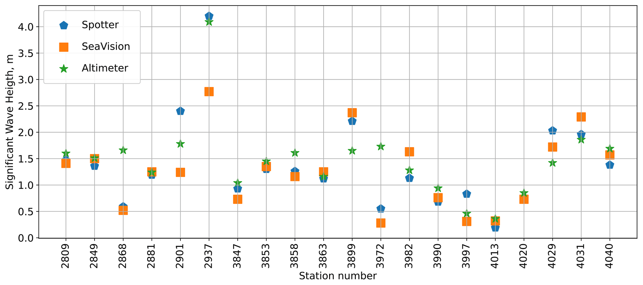
Figure 9 Significant wave height estimates for the locations of satellite altimeter overpasses for three research cruises. Numbers on the horizontal axis correspond to the station numbering in Table A1.

4 Data availability

Datasets that contain significant wave heights, wave periods, wave directions, wave energy frequency spectra, meteorological data, and other related parameters from both SeaVision and the Spotter buoy at the locations of every station (Table A1) are available in the PANGAEA repository – https://doi.org/10.1594/PANGAEA.939620 (Gavrikov et al., 2021). In this dataset we provide wind wave statistics disregarding separation of the swell and wind waves at this stage of the SeaVision development. We plan to include this procedure in the next studies. At the same time, we provide a 1D spectrum that potentially allows us to see the first and second peaks associated with wind waves and swell (an example is shown in Fig. 4b). Users interested in the analysis of the raw radar dataset or in the wave characteristics in the locations where measurements were carried out only with SeaVision are welcome to request access from Alexander Gavrikov (gavr@sail.msk.ru).

5 Conclusions

To broaden the avenue for widely needed broad-scale high-quality observations of ocean wind wave estimates, we used a conventional navigation X-band ship radar equipped with a SeaVision recorder and software package. Here we present the evaluation of the instrument package for measuring wind wave parameters and comparing them to in situ observations and model results. The data were collected on three cruises in the subpolar North Atlantic and in the Kara Sea. All SeaVision records were co-located with in situ Spotter buoy measurements, which were used for validation. We demonstrate overall agreement of the estimates of significant wave height and wave period measured by SeaVision with the Spotter buoy measurements and with simulations using the WW3 spectral wave model. Estimates of significant wave height between SeaVision, WW3, and the Spotter buoy are in better agreement than those for the wave periods. In the ranges of H_s up to 4.2 m the average difference between the Spotter buoy and SeaVision is around 10 cm for H_s, while WW3 simulations are lower than SeaVision H_s by 28 cm. We note, however, that comparisons to WW3 should be considered with caution, as the model results are significantly dependent on the choice of forcing function (atmospheric reanalysis). SeaVision tends to underestimate mean wave periods by ∼0.5 s compared to the Spotter buoy, while the differences in periods with WW3 simulations may amount to more than 2 s. Also, very good agreement was found for the wave directions, whose spread across all three data sources does not exceed 10^∘.

We present the newly developed SeaVision system for digitizing and recording the analogue signals from navigation radars and further providing quantitative estimates of wind wave characteristics. A broad implementation of SeaVision opens a potential for enhancing massive observations of wind waves over the open ocean. SeaVision is currently mounted on board two R/Vs operated by IORAS, but in 2022 five more IORAS R/Vs will be supplied with SeaVision systems. Data records will become operationally available on an open-source web page. In 2023 we also plan to develop a portable and cheaper version of SeaVision that can be easily mounted on board any commercial ship with navigational radar operating in the open ocean as well as on the platform, lighthouse, or any coastal infrastructure. After further validation in different sea state and weather conditions, we plan to upgrade SeaVision to a portable device and to incorporate all post-processing procedures into the internal software package that will make it possible for commercial ships on which the system is installed to provide real-time reporting of wind wave parameters through the Global Telecommunication System (GTS). Theoretically the estimated data flow is formally one estimate per 2–3 s (one full turn of the radar antenna). Even with a reporting frequency of once per minute, the potential of the SeaVision data flow exceeds the current VOS data flow by 100 times. Contrasting with existing commercial systems for wind wave monitoring with navigational marine radars, such as WaMoS II (http://www.oceanwaves.de, last access: 4 August 2022), SeaDarQ (http://www.seadarq.com/seadarq?set_language=en, last access: 4 August 2022), and WaveFinder (Park et al., 2006), SeaVision represents potentially a low-cost, portable, and easy-to-install alternative. Wide use of such a system on commercial ships can drastically increase the number of sea state observations available to users, including the National Meteorological Offices using this information as data assimilation input for NWP models and reanalyses. The Global Climate Observing System (GCOS) and associated Global Ocean Observing System (GOOS) consider the sea state to be a critical climate variable highly demanded by global observing modules. We hope that SeaVision with its perspective to provide exceptionally high global coverage with online wave measurements will meet this urgent demand and help to satisfy GCOS given its mandate for systematic observations under the UN Framework Convention on Climate Change (UNFCCC), also including GCOS and GOOS responsibilities under the Subsidiary Body for Scientific and Technological Advice (SBSTA) and the Subsidiary Body for Implementation (SBI).

Appendix A: List of the locations (stations) of the wind wave measurements during three research cruises

Table A1 Stations list: geographical locations and time of all stations where the wind wave measurements were performed simultaneously with SeaVision and the Spotter buoy. In the last column letters stand for the name of the research vessel (ASV – Akademik Sergey Vavilov, AI – Akademik Ioffe) and numbers stand for the sequence number of a research cruise since the beginning of the research vessel operation.

Appendix B: Methodology for the computation of wave parameters from sea clutter images

We stated above (Sect. 2.2.2) that, to relate the signal to the wind waves, we assume that components of the spectrum outside of the dispersion relation are related to the background speckle noise and components of the spectrum that satisfy the dispersion relation Eq. (1) related to the signal, associated with the wind waves. Equation (1) presents the dispersion relation for the first harmonic and can also be easily extended to the second harmonic as follows:

$$\begin{array}{}\text{(B1)}& {\mathit{\omega }}_{n,\mathrm{2}}\left(k\right)=\sqrt{\mathrm{2}gk}+\mathrm{2}k\cdot U\cdot \cos {\mathit{\theta }}_n.\end{array}$$

Here and later index n refers to the number of the directional sector (22.5^∘ width each). The curve associated with the second harmonic is clearly seen in Fig. 3. The rest of the signal lying in the spectral domain outside the bands associated with dispersion curves and attributed to speckle noise (Kanevsky, 2009) is needed to be properly quantified. This depends on the algorithm used for the quantification of bands associated with dispersion relation curves. Speckle noise is used for normalization of the radar spectrum and removal of the impulse power impact on the radar signal modulations by the sea waves (Kanevsky, 2009). The 2D normalized spectrum $S_{n,\mathrm{2}\mathrm{d},\mathrm{norm}}\left(kf\right)$ of the signal at each wavenumber k can be calculated as

$$\begin{array}{}\text{(B2)}& S_{n,\mathrm{2}\mathrm{d},\mathrm{norm}}\left(k,f\right)={\displaystyle \frac{S_{n,\mathrm{2}\mathrm{d},\mathrm{image}}(k,f)}{\int S_{n,\mathrm{2}\mathrm{d},\mathrm{image},\mathit{\omega }\mathrm{speckle}}\left(k,f\right)\mathrm{d}f}},\end{array}$$

where the speckle frequency is

$$\begin{array}{}\text{(B3)}& {\mathit{\omega }}_{\mathrm{speckle}}=(f\notin {\mathit{\omega }}_{n,\mathrm{1}}/\mathrm{2}\mathit{\pi }\mathrm{and}f\notin {\mathit{\omega }}_{n,\mathrm{2}}/\mathrm{2}\mathit{\pi }).\end{array}$$

Then the full image spectrum $S_{n,\mathrm{1},\mathit{\omega }}\left(f\right)$ needs to be filtered to obtain the power corresponding to the band capturing the first ω_n,1 harmonic for the direction n:

$$\begin{array}{}\text{(B4)}& S_{n,\mathrm{1},\mathit{\omega }}\left(f\right)={\int }_{k_n,\mathrm{1}-\mathrm{\Delta }k}^{k_{n,\mathrm{1}}+\mathrm{\Delta }k}{S}_{n,\mathrm{2}\mathrm{d},\mathrm{norm}}\left(k,f\right)\mathrm{d}k.\end{array}$$

Here k_n,1 is the dispersion relation Eq. (1) solution for the first harmonic ${\mathit{\omega }}_{n,\mathrm{1}}\left(k_{n,\mathrm{1}}\right)=\mathrm{2}\mathit{\pi }f$ and Δk is related to the size of the processing area (720 m) as $\mathrm{\Delta }k=\mathrm{0.02}\approx \mathrm{2}\cdot \mathrm{2}\mathit{\pi }/\mathrm{720}$ (rad m⁻¹). Similarly, for the second harmonic ω_n,2, we obtain

$$\begin{array}{}\text{(B5)}& S_{n,\mathrm{2},\mathit{\omega }}\left(f\right)={\int }_{k_{n,\mathrm{2}}-\mathrm{\Delta }k}^{k_{n,\mathrm{2}}+\mathrm{\Delta }k}{S}_{n,\mathrm{2}\mathrm{d},\mathrm{norm}}(k,f)\mathrm{d}k,\end{array}$$

where k_n,2 is the dispersion relation Eq. (B1) solution for the second harmonic ${\mathit{\omega }}_{n,\mathrm{2}}\left(k_{n,\mathrm{2}}\right)=\mathrm{2}\mathit{\pi }f$.

The total power S_n,ω(f) falling in the bands along dispersion relation curves yields

$$\begin{array}{}\text{(B6)}& S_{n,\mathit{\omega }}\left(f\right)=S_{n,\mathrm{1},\mathit{\omega }}\left(f\right)+S_{n,\mathrm{2},\mathit{\omega }}\left(f\right).\end{array}$$

Given that this procedure is applied to all 16 sectors of the image (see Sect. 2.2.2), the omnidirectional image frequency spectrum S_image(f) can be derived as follows:

$$\begin{array}{}\text{(B7)}& S_{\mathrm{image}}\left(f\right)={\displaystyle \frac{\mathrm{1}}{\mathrm{16}}}{\sum }_{n=\mathrm{1}}^{\mathrm{16}}{S}_{n,\mathit{\omega }}\left(f\right).\end{array}$$

Further integration over the frequency domain returns the zeroth moment m_0,image of the S_image(f) spectrum:

$$\begin{array}{}\text{(B8)}& m_{\mathrm{0},\mathrm{image}}={\int }_{f{r}^{\mathrm{8}}}^{f{r}^{\mathrm{48}}}{S}_{\mathrm{image}}\left(f\right)\mathrm{d}f,\end{array}$$

which provides us with the estimate of the SNR:

$$\mathrm{SNR}\equiv m_{\mathrm{0},\mathrm{image}}+\mathrm{1}.$$

The limits of the integration in Eq. (B8) are fr⁸=8Δf and fr⁴⁸=48Δf, where $\mathrm{\Delta }f=\frac{\mathrm{rpm}}{\mathrm{60}\cdot \mathrm{48}}$ is defined by the antenna rotation speed rpm (rotations per minute, Table 2) and the 48-point size window of FT in the time domain.

Formally, considering the S_image(f) spectrum to be a modulation analogue of the real sea wave spectrum, S_w(f), the zeroth moment m_0,image can be further converted to the magnitude of signal modulations H_image in the radar image, which stands as a provisional measure of H_s:

$$\begin{array}{}\text{(B9)}& H_{\mathrm{image}}=\mathrm{4}\sqrt{m_{\mathrm{0},\mathrm{image}}}.\end{array}$$

Further, the transform of the omnidirectional SeaVision image frequency spectrum S_image(f) to the sea wave frequency (wave energy) spectrum S_w,SeaVision(f) visible by SeaVision is performed by applying the standard technique described in Sect. 2.2.2 and resulting in Eq. (2) returning significant wave height H_s,SeaVision estimates based on the radar calibration coefficients A and B along with estimates for the wind wave period Eq. (3) derived from the zeroth and first moments of the spectrum.

The mean wave direction D_s,SeaVision is estimated with the centroid method:

$$\begin{array}{}\text{(B10)}& {\displaystyle }{D}_{\mathrm{s},\mathrm{SeaVision}}={\displaystyle \frac{\mathrm{180}}{\mathit{\pi }}}\arg \left({\displaystyle \frac{{\sum }_{n=\mathrm{1}}^{\mathrm{16}}\exp \left(i\frac{\mathit{\pi }}{\mathrm{180}}{\mathit{\theta }}_n\right)D_n}{\sum _{n=\mathrm{1}}^{\mathrm{16}}{D}_n}}\right),\text{(B11)}& {\displaystyle }{D}_n={\int }_{f{r}^{\mathrm{8}}}^{f{r}^{\mathrm{48}}}{S}_{n,\mathit{\omega }}\left(f\right)\mathrm{d}f,\end{array}$$

where arg is the argument of the complex number and D_n is the zeroth moment of the spectrum S_n,ω(f) in the direction n.

Appendix C

Table C1 Definition of all the parameters in the paper and dataset.